Exam 2: Exploring Relationships Between Variables

The model ) can be used to predict the stopping distance (in feet) for a Car traveling at a specific speed (in mph). According to this model, about how much distance will a Car going 65 mph need to stop?

The relationship between the number of hours a person practices a task and the time it takes them To complete the task is calculated to have R $\mathrm { R } - \mathrm { sq } = 56.7 \%$ ) The value of the correlation coefficient is

If a data point is influential it…

Email At CPU every student gets a college email address. Data collected by the college showed a negative association between student grades and the number of emails the student sent during the semester. a. Briefly explain what "negative association" means in this context. b. After seeing this study the college proposes trying to improve academic performance by limiting the amount of email students can send through the college address. As a statistician, what do you think of this plan? Explain briefly.

All but one of the statements below contain a mistake. Which one could be true?

A scatterplot of log(Y) vs. log(X) reveals a linear pattern with very little scatter. It is probably true That …

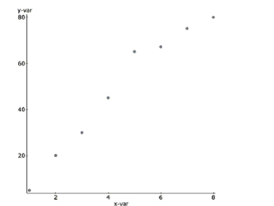
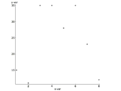
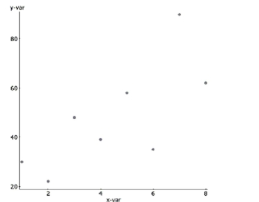
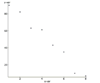
Match each graph with the appropriate correlation coefficient. _____ 0.98 _____ 0.73 _____ 0.09 _____ -0.99 A. B. C. D.

A silly psychology student gathers data on the shoe size of 30 of his classmates and their GPA's. The correlation coefficient between these two variables is most likely to be

Although there are annual ups and downs, over the long run, growth in the stock market averages About 9% per year. A model that best describes the value of a stock portfolio is probably:

Carbon dating QuarkNet, a project funded by the National Science Foundation and the U.S. Department of Energy, poses the following problem on its website: "Last year, deep within the Soudan mine, QuarkNet teachers began a long-term experiment to measure the amount of carbon-14 remaining in an initial 100-gram sample at 2000-year intervals. The experiment will be complete in the year 32001. Fortunately, a method for sending information backwards in time will be discovered in the year 29998, so, although the experiment is far from over, the results are in." Here is a portion of the data: Time (yr) 0 2000 4000 6000 8000 10,000 12,000 14,000 16,000 18,000 Mass (g) 100 76 61 47 36 29 22 17 13 10 A scatterplot of these data looks like: 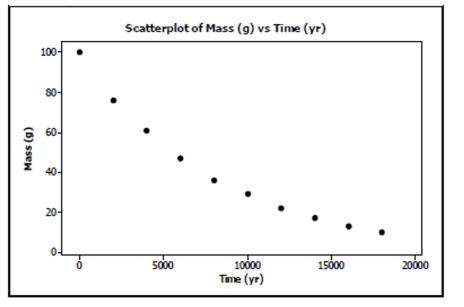a. Straighten the scatterplot by re-expressing these data and create an appropriate model for predicting the mass from the year. b. Use your model to estimate what the mass will be after 7500 years. c. Can you use your model to predict when 50 g of the sample will be left? Explain.

Time Wasted A group of students decide to see if there is link between wasting time on the internet and GPA. They don't expect to find an extremely strong association, but they're hoping for at least a weak relationship. Here are the findings. linear regression results: Dependent Variable: GPA Sample size: 10 R (correlation coefficient) =-0.37199274 R-sq =0.1383786 s=0.85365134 Parameter Estimate Std. Err. Intercept 4.06191 0.74405 Hours/week -0.0297 0.02616 a. How strong is the relationship the students found? Describe in context with statistical justification. One student is concerned that the relationship is so weak, there may not actually be any relationship at all. To test this concern, he runs a simulation where the 10 GPA's are randomly matched with the 10 hours/week. After each random assignment, the correlation is calculated. This process is repeated 100 times. Here is a histogram of the 100 correlations. The correlation coefficient of -0.371 is indicated with a vertical line. 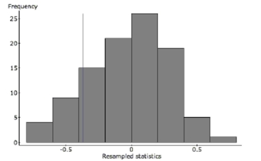b. Do the results of this simulation confirm the suspicion that there may not be any relationship? Refer specifically to the graph in your explanation.

Halloween is a fun night. It seems that older children might get more candy because they can travel further while trick-or-treating. But perhaps the youngest kids get extra candy because they are so cute. Here are some data that examine this question, along with the regression output. Dependent Variable: candy Sample size: 9 $R ($ correlation coefficient $) = 0.19534425$ R-sq=0.038159375 s=11.297554 Parameter Estimate Std. Err. Intercept 13.569231 9.0783516 Age 3.4038462 1.0175376 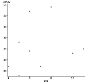-Based on the graph and the regression output, what conclusions do you draw regarding the relationship between age and the number of pieces of candy a trick-or-treater collects?

During a science lab, students heated water, allowed it to cool, and recorded the temperature over time. They computed the difference between the water temperature and the room temperature. The results are in the table. Time (in minutes) 10 20 30 40 50 60 Difference in temp. (degrees F) 68 36 20 10 6 4 -Use the equation = 2.057 - 0.025\) time to predict the difference in temperature after 45 minutes.

Two variables that are actually not related to each other may nonetheless have a very high Correlation because they both result from some other, possibly hidden, factor. This is an example of

To achieve linearity, the data was transformed using a square root function of cost. Here are the results and a residual plot. Dependent Variable: sqrt(cost) $\mathrm { R }$ (correlation coefficient) $= \mathbf { 0 . 9 8 9 4 6 6 2 7 }$ -=0.97904349 :0.2141 Parameter coeff se Intercept 1.1857 0.4346 height 0.1792 0.0151 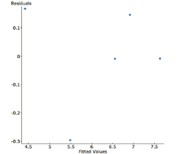-Write the transformed regression equation. Make sure to define any variables used in your equation.

An article in the Journal of Statistics Education reported the price of diamonds of different sizes in Singapore dollars (SGD). The following table contains a data set that is consistent with this data, adjusted to US dollars in 2004: 2004 US \ Carat 494.82 0.12 768.03 0.17 1105.03 0.20 1508.88 0.25 1826.18 0.28 2096.89 0.33 2004 US \ Carat 688.24 0.15 944.90 0.18 1071.75 0.21 1504.44 0.26 1908.28 0.29 2409.76 0.35 V -Interpret the slope of your model in context.

The following is a scatterplot of the average final exam score versus midterm score for 11 sections of an introductory statistics class: 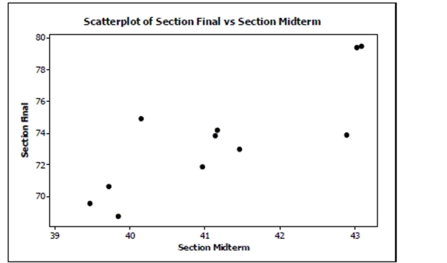The correlation coefficient for these data is $r = 0.829$ 29. If you had a scatterplot of the final exam score versus midterm score for all individual students in this introductory statistics course, would the correlation coefficient be weaker, stronger, or about the same? Explain.

If r = -0.4 for the relationship between the time of day and amount of coffee in an office worker's Mug, which are true? I. $r ^ { 2 } = - 16 \%$ II. There is a linear relationship between time and amount of coffee. III. 16% of the variability is correctly predicted by time of day.

It takes a while for new factory workers to master a complex assembly process. During the first Month new employees work, the company tracks the number of days they have been on the job and The length of time it takes them to complete an assembly. The correlation is most likely to be

Baseball coaches use a radar gun to measure the speed of pitcher's fastball. They also record outcomes such as hits and strikeouts. The scatterplot below shows the relationship between the average speed of a fastball and the average number of strikeouts per nine innings for each pitcher on the Bulldogs, based on the past season. 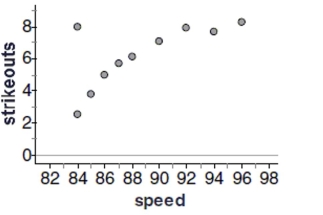-Comment on any unusual data point or points in the data set. Explain.