Exam 8: Regression, Associations, and Predictive Modeling
A survey of families revealed that 58% of all families eat turkey at holiday meals, 44% eat
ham, and 16% have both turkey and ham to eat at holiday meals.
a. What is the probability that a family selected at random had neither turkey nor ham at
their holiday meal?
b. What is the probability that a family selected at random had only ham without having
turkey at their holiday meal?
c. What is the probability that a randomly selected family having turkey had ham at their
holiday meal?
d. Are having turkey and having ham disjoint events? Explain.
![a. P (neither ham nor turkey) = 1 - P ( ham or turkey ) = 1 - [ P ( ham ) + P (turkey) - P ( ham and turkey ) ] = 1 - [ 0.44 + 0.58 - 0.16 ] = 1 - 0.86 = 0.14 Or, using the Venn diagram, 14\% b. P ( ham only ) = P ( ham ) - P ( ham and turkey ) = 0.44 - 0.16 = 0.28 Or, using the Venn diagram, 28 \% c. P ( ham I turkey ) = \frac { P ( \text { ham and turkey } ) } { P ( \text { turkey } ) } = \frac { 0.16 } { 0.58 } = 0.2759 d. No, the events are not disjoint, since some families ( 16 \% ) have both ham and turkey at their holiday meals.](https://storage.examlex.com/TB3452/11ecdc0a_921f_6ff9_82f6_df69db8665c4_TB3452_11.jpg)
a. (neither ham nor turkey)
ham or turkey
ham (turkey) ham and turkey
Or, using the Venn diagram, 14\%
b. ham only ham ham and turkey
Or, using the Venn diagram,
c. ham I turkey
d. No, the events are not disjoint, since some families have both ham and turkey at their holiday meals.
Homelessness is a problem in many large U.S. cities. To better understand the problem, a
multiple regression was used to model the rate of homelessness based on several
explanatory variables. The following data were collected for 50 large U.S. cities. The
regression results appear below. Homeless number of homeless people per 10,000 in a city Poverty percent of residents with income under the poverty line Unemployment percent of residents unemployed Temperature average yearly temperature (in degrees .)
Vacancy percent of housing that is unoccupied Rent Control indicator variable, 1= city has rent control, 0= no rent control
Dependent variable is Homeless
squared squared (adjusted)
with degrees of freedom
Variable Coeff SE(Coeff) t-ratio p-value Constant -4.275 3.465 -1.23 0.2239 Poverty 0.0823 0.0823 1.00 0.3228 Unemployment 0.159 0.218 0.73 0.4699 Temperature 0.135 0.0587 2.30 0.0262 Vacancy -0.247 0.138 -1.79 0.0809 Rent Control 2.944 1.37 2.15 0.0373
a. Using a 5% level of significance, which variables are associated with the number of
homeless in a city?
b. Explain the meaning of the coefficient of temperature in the context of this problem.
c. Explain the meaning of the coefficient of rent control in the context of this problem.
d. Do the results suggest that having rent control laws in a city causes higher levels of
homelessness? Explain.
e. If we created a new model by adding several more explanatory variables, which statistic
should be used to compare them
f. Using the plots below, check the regression conditions. 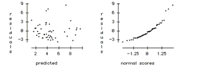
a. Temperature and Rent Control
b. For cities with similar values for the other explanatory variables (poverty, unemployment, etc.), on average, each additional degree of average yearly temperature is associated with an increase of homeless people per 10,000 residents of the city.
c. For cities with similar values of the other explanatory variables (poverty, unemployment, etc.), cities with rent control laws have, on average, more homeless people per 10,000 residents than cities without rent control laws. d. No. This is an observational study, so the results cannot be used to establish cause-and-effect. There is evidence that cities with rent control laws are associated with higher levels of homelessness, but the cause may not be the rent control laws themselves.
e. The adjusted should be used to compare regression models because the models have different numbers of predictor variables.
f. * Straight enough condition: OK. The plot of residuals vs. predicted values shows no obvious curvature. (We should also check plots of Homeless vs. each X variable.) * Does the plot thicken? condition: OK. The plot of residuals vs. predicted values is approximately the same width throughout.
* Randomization condition: Caution. We do not know whether or not the 50 U.S. cities in our sample were chosen randomly, or whether they are representative of all large U.S. cities.
* Nearly Normal condition: Violated. The normal probability plot is curved, which indicates that the regression errors do not follow a Normal model. (It may be possible to re-express the -variable to fix this problem.)
Dice rolls Two players compete against each other by rolling dice - not the traditional
dice, though. One face of Alphonso's die has an 8 and the other five faces are all 2's.
Bettina's die has four 3's and two 1's on the six faces.
a. They each roll their die, and the player with the highest score wins. Which player has the
advantage? Explain.
b. If Alphonso wins, Bettina pays him $10. How much should he pay her if she wins in
order to make the game fair?
c. They decide to change the rules. They'll each roll, and the winner will collect the number
of dollars shown on his or her die. For example, If Alphonso rolls a 2 and Bettina rolls a 3,
he'll pay her $3. Create a probability model for the amount Alphonso wins.
d. Find the expected value and standard deviation of Alphonso's winnings at this game.
e. If they play this new game repeatedly which player has the advantage? Explain.
C.
d.
Standard deviation
e. Alphonso has the advantage, because his expected value is positive. He expects to win an average of for each time they play the game.
Would it make sense to have a control group that did not get any of the treatments
described above?
Do you think there is a clear pattern? Describe the association between fiber and calories.
The distribution below is the number of family members reported by 25 people in the 2010 Census.
The best description for the shape of this distribution is 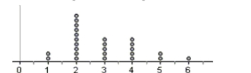
On a physical fitness test middle school boys are awarded one point for each push-up they can do,
And a point for each sit-up. National results showed that boys average 18 pushups with a standard
Deviation of 4 push-ups, and 34 sit-ups with standard deviation 11. The mean of their combined
(total) scores was therefore 1
Points. What is the standard deviation of their combined
Scores?
Traffic accidents Police reports about the traffic accidents they investigated last year
indicated that 40% of the accidents involved speeding, 25% involved alcohol, and 10%
involved both risk factors.
a. What is the probability that an accident involved neither alcohol nor speed?
b. Do these two risk factors appear to be independent? Explain.
Nickels minted in the United States are supposed to weigh 5.000 grams. Of course there is
some variation in that. The actual weights are pretty well represented by a normal model
with a mean of 5.000 g and a standard deviation of about 0.08 g. Draw and clearly label this
model. 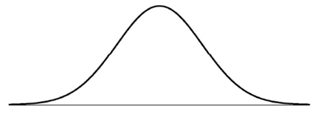
What is the probability that if he removes 2 marbles without looking, that he will get two
orange marbles?
Cellphones ConsumerReports.org evaluated the price and performance of 99 models of
cellphones. Computer output gives these summaries for the prices: Min Q1 Median Q3 Max MidRange Mean TrMean SD 0 0 50 200 400 200 96.36 90.21 107.23
a. Were any of the prices outliers? Explain how you made your decision.
b. One of the manufacturers advertises a cellphone "economy-priced at only $31.95".
Would you consider that to be a very low price? Explain.
A study by a prominent psychologist found a moderately strong positive association
between the number of hours of sleep a person gets and the person's ability to memorize
information.
a. Explain in the context of this problem what "positive association" means.
b. Hoping to improve academic performance, the psychologist recommended the school
board allow students to take a nap prior to any assessment. Discuss the psychologist's
recommendations.
What is the probability that at least 3 of the first 40 customers buy specialty clothes for their
pet? Show work.
In this context describe a Type II error and the impact such an error would have on the
store.
The Postmaster of a city's Post Office believes that a Normal model is useful in projecting
the number of letters which will be mailed during the day. They use a mean of 20,000
letters and a standard deviation of 250 letters. Draw and clearly label this model. 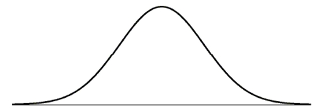
Which of the following is true about Type I and Type II errors?
I. Type I errors are always worse than Type II errors.
II. The severity of Type I and Type II errors depends on the situation being tested.
III. In any given situation, the higher the risk of Type I error, the lower the risk of Type II error.
A statistics teacher gave her class a 15 point quiz. The summary statistics for the students'
scores are shown in the table. 10.95 points s 2.481 points min 4 Q1 9.5 median 12 Q3 12 15
a. Notice that the median score and the third quartile are the same. Explain how this can
be.
b. One student's parent heaped praise on him for scoring 13, saying it was an amazing
score. Comment on whether that praise is deserved using the summary statistics as
support.
c. To convert these raw scores to a score out of 100, the teacher multiplies each score by six,
then adds 10. (We can debate the wisdom of such a strategy later!). What is the median
converted score? And the IQR?
d. What are the mean and standard deviation of the converted test scores?
We have calculated a confidence interval based on a sample of size n = 100. Now we want to get a
Better estimate with a margin of error that is only one-fourth as large. How large does our new
Sample need to be?
A correlation of zero between two quantitative variables means that
Filters
- Essay(0)
- Multiple Choice(0)
- Short Answer(0)
- True False(0)
- Matching(0)