Exam 7: Inference When Variables Are Related

Of the 23 first year male students at State U. admitted from Jim Thorpe High School, 8 were offered baseball scholarships and 7 were offered football scholarships. The University admissions committee looked at the students' composite ACT scores (shown in the tabl, wondering if the University was lowering their standards for athletes. Assuming that this group of students is representative of all admitted students, what do you think? 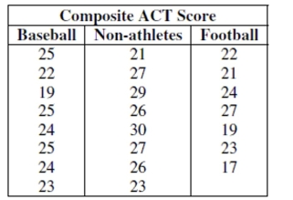-Test an appropriate hypothesis and state your conclusion.

Engineers want to know what factors are associated with gas mileage. The regression below predicts the average miles per gallon (MPG) for 82 cars using their engine horsepower (HP) and weight (WT, in 100's of pounds). Dependent variable is MPG $R$ squared $= 82.4 \% \quad$ R squared (adjusted) $= 81.9 \%$ $s = 4.255$ with $82 - 3 = 79$ degrees of freedom 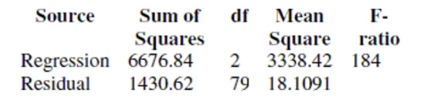Variable Coeffcient SE(Coeff) t-ratio p-value Constant 66.855 2.079 32.2 <0.0001 HP -0.0209708 0.015 -1.4 0.1661 WT -0.990369 0.1047 -9.45 <0.0001 a. Write down the regression equation. b. Write down the hypotheses for the test of the coefficient of horsepower. Conduct the test and explain your conclusion in the context of this problem. c. Write down the hypotheses for the test of the coefficient of weight. Conduct the test and explain your conclusion in the context of this problem. d. Explain the meaning of the coefficient of weight in the context of this problem. e. Explain the meaning of the intercept of this regression in the context of this problem. f. Compute the predicted gas mileage of a 3500 pound car with a 150 horsepower engine. The plots are MPG vs. HP, MPG vs. WT, residuals vs. predicted values, and a normal probability plot of residuals. 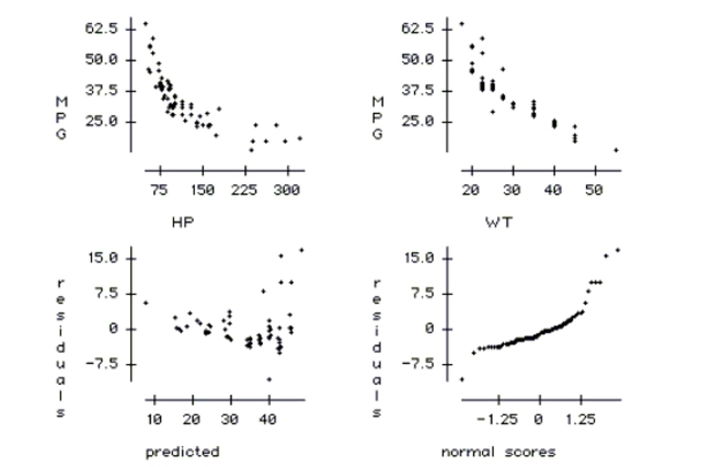g. Check the conditions of this regression and comment on whether they are satisfied.

Here are data about the average January low temperature in cities in the United States, and factors that might allow us to predict temperature. The data, available for 55 cities, includ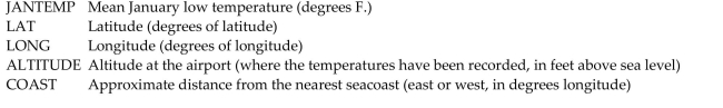e: We will attempt to make a regression model to help account for mean January temperature and to understand the effects of the various predictors. At each step of the analysis you may assume that things learned earlier in the process are known. Units Note: The "degrees" of temperature, given here on the Fahrenheit scale, have only coincidental language relationship to the "degrees" of longitude and latitude. The geographic "degrees" are based on modeling the Earth as a sphere and dividing it up into 360 degrees for a full circle. Thus 180 degrees of longitude is halfway around the world from Greenwich, England (0°) and Latitude increases from 0 degrees at the Equator to 90 degrees of (North) latitude at the North Pole. 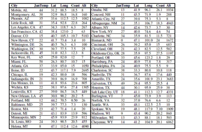-Here is a partial regression plot for the coefficient of Long in the regression with a least squares regression line added to the display: 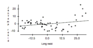What is the slope of the line on this display? Does the display suggest that this slope adequately summarizes the effect of longitude in the regression? Why/Why not?

In ANOVA, an interaction between two factors means that…

Here are data about the average January low temperature in cities in the United States, and factors that might allow us to predict temperature. The data, available for 55 cities, includ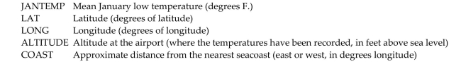e: We will attempt to make a regression model to help account for mean January temperature and to understand the effects of the various predictors. At each step of the analysis you may assume that things learned earlier in the process are known. Units Note: The "degrees" of temperature, given here on the Fahrenheit scale, have only coincidental language relationship to the "degrees" of longitude and latitude. The geographic "degrees" are based on modeling the Earth as a sphere and dividing it up into 360 degrees for a full circle. Thus 180 degrees of longitude is halfway around the world from Greenwich, England (0°) and Latitude increases from 0 degrees at the Equator to 90 degrees of (North) latitude at the North Pole. 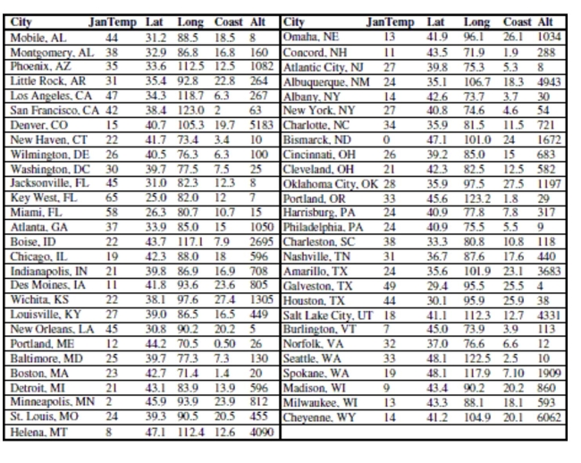-First, we consider the relationship between temperature and latitude. This seems to be the obvious first choice; everybody knows that northern (high latitude) cities tend to be colder in January than southern (lower latitude) cities. Here is the scatterplot: 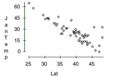Describe what you see in this scatterplot in a sentence or two. Which of the regression assumptions for the regression of Jantemp on Lat can you check with this plot? State them and indicate whether you think they seem to be satisfied.