Exam 13: Inference in Linear Models

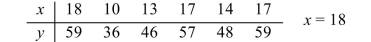
In a study of reaction times, the time to respond to a visual stimulus (x) and the time to respond to an auditory stimulus (y) were recorded for each of 8 subjects. Times were measured in thousandths of A second. The results are presented in the following table. Visual Auditory 185 244 204 244 242 247 209 245 191 243 250 249 155 237 188 245 Compute a point estimate for the mean auditory response time for subjects with a visual response time of .

In a study of reaction times, the time to respond to a visual stimulus (x) and the time to respond to an auditory stimulus (y) were recorded for each of 8 subjects. Times were measured in thousandths of A second. The results are presented in the following table. Visual Auditory 166 241 192 242 242 250 188 244 232 252 240 254 197 245 203 247 Predict the auditory response time for a particular subject whose visual response time of 178.

In a study of reaction times, the time to respond to a visual stimulus (x) and the time to respond to an auditory stimulus (y) were recorded for each of 8 subjects. Times were measured in thousandths of a second. The results are presented in the following table. Visual Auditory 168 243 233 253 169 242 204 243 206 248 202 245 157 239 240 248 i). Compute a point estimate for the mean auditory response time for subjects with a visual response time of 183. ii). Construct a 99% confidence interval for the mean auditory response time for subjects with a visual response time of 183. iii). Predict the auditory response time for a particular subject whose visual response time of 183. iv). Construct a 99% prediction interval for the auditory response time for a particular subject whose visual response time is 183.

The following display from a TI-84 Plus calculator presents the results of a test of the null hypothesis 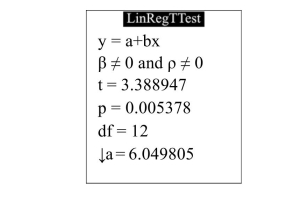$H _ { 0 } : \beta _ { 1 } = 0$ . What is the value of the test statistic?

The summary statistics for a certain set of points are: $n = 12 , s _ { \mathrm { e } } = 3.505 , \quad \sum ( x - \bar { x } ) ^ { 2 } = 14.353$ , and $b _ { 1 } = 1.560$ Assume the conditions of the linear model hold. A 95% confidence interval for $\beta _ { 1 }$ will be constructed. Construct the 95% confidence interval.

The following MINITAB output presents a multiple regression equatior $\hat { y }$ =b₀+b₁x₁+b₂x₂+b₃x₃+b₄x₄ The regression equation is $\mathrm { Y } = 4.7712 + 0.2662 \mathrm { X } 1 + 1.2710 \mathrm { X } 2 - 1.1349 \mathrm { X } 3 - 1.8545 \mathrm { X } 4$ Predictor Coef SE Coef T Constant 4.7712 0.7648 0.92800 0.3280 1 0.2662 0.8036 -0.93740 0.3570 2 1.2710 0.8451 1.74170 0.0830 3 -1.1349 0.6318 -2.94990 0.0080 4 -1.8545 0.6753 3.27200 0.0020 $\text { Analysis of Variance }$ Source DF SS MS F P Regression 4 624.2 156.1 9.8797 0.003 Residual Error 40 633.7 15.8 Total 44 1,257.9 It is desired to drop one of the explanatory variables. Which of the following is the most appropriate action?

The summary statistics for a certain set of points are: $n = 17 , s _ { \mathrm { e } } = 2.880 , \sum ( x - \bar { x } ) ^ { 2 } = 19.241$ , and $b _ { 1 } = 1.839$ . Assume the conditions of the linear model hold. A $95 \%$ confidence interval for $\beta _ { 1 }$ will be constructed. What is the margin of error?

Use the given set of points to construct a $95 \%$ confidence interval for the mean response for the given value of $x$ .

In a study of reaction times, the time to respond to a visual stimulus (x) and the time to respond to an auditory stimulus (y) were recorded for each of 8 subjects. Times were measured in thousandths Of a second. The results are presented in the following table. Visual Auditory 208 249 200 244 245 254 234 249 155 243 211 248 189 244 206 247 Test H₀: $\beta _ { 1 }$ =0 versus $\beta _ { 1 } \neq 0$ . Use the $\alpha$ :=0.05 level of significance.

The following display from a TI-84 Plus calculator presents the results of a test of the null hypothesis 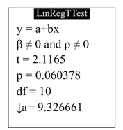$H _ { 0 } : \beta _ { 1 } = 0$ Can you conclude that the explanatory variable is useful in predicting the outcome variable? Answer this question using the $\alpha = 0.05$ level of significance.

The following display from a TI-84 Plus calculator presents the results of a test of the null hypothesis 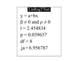$H _ { 0 } : \beta _ { 1 } = 0$ . What is the P-value?

For a sample of size 15 , the following values were obtained: $b _ { 0 } = 3.58 , b _ { 1 } = 4.79 , s _ { \mathrm { e } } = 4.09$ , $\sum ( x - \bar { x } ) ^ { 2 } = 237.89$ , and $\bar { x } = 3.00$ Construct a $95 \%$ confidence interval for the mean response when $x = 0$ .

The summary statistics for a certain set of points are: $n = 23 , s _ { \mathrm { e } } = 2.302 , \sum ( x - \bar { x } ) ^ { 2 } = 15.372$ , and $b _ { 1 } = 1.902$ . Assume the conditions of the linear model hold. A $99 \%$ confidence interval for $\beta _ { 1 }$ will be constructed. How many degrees of freedom are there for the critical value?

Use the given set of points to a). Compute $b _ { 0 }$ and $b _ { 1 }$ . b). Compute the predicted value $\hat { y }$ for the given value of x. c). Compute the residual standard deviation $s _ { \mathrm { e } }$ d). Compute the sum of squares for $x , \quad \sum ( x - \bar { x } ) ^ { 2 }$ e). Find the critical value for a 95% confidence or prediction interval. f). Construct a 95% confidence interval for the mean response for the given value of x. g). Construct a 95% prediction interval for an individual response for the given value of x. x 12 10 19 15 11 15 y 31 28 46 39 31 37 xequals16

The summary statistics for a certain set of points are: n=10, s_e=3.199, $\sum { ( x - \bar { x } ) ^ { 2 } }$ =11.257, and $\beta _ { 1 }$ =1.704 . Assume the conditions of the linear model hold. A 99% confidence interval for $\beta _ { 1 }$ will be constructed. i). How many degrees of freedom are there for the critical value? ii). What is the critical value? iii). What is the margin of error? iv). Construct the 99% confidence interval.

In a study of reaction times, the time to respond to a visual stimulus (x) and the time to respond to an auditory stimulus (y) were recorded for each of 6 subjects. Times were measured in thousandths of A second. The results are presented in the following table. The following MINITAB output describes the fit of a linear model to these data. Assume that the assumptions Of the linear model are satisfied. The regression equation is Auditory $= 169.803813 + 0.4671$ Visual Predictor Coef SE Coef T P Constant 169.803813 17.123244 9.916568 0.000581 Visual 0.4671 0.081367 5.740635 0.004563 What is the slope of the least-squares regression line?

The following MINITAB output presents a confidence interval for a mean response and a prediction interval for an individual response. 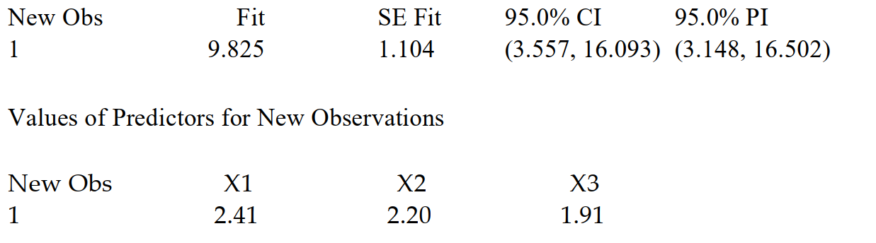What is the $95 \%$ prediction interval for the new observation?

The following MINITAB output presents a 95% confidence interval for the mean ozone level on days when the relative humidity is 40%, and a 95% prediction interval for the ozone level on a Particular day when the relative humidity is 40%. The units of ozone are parts per billion. Predicted Values for New Observations New Obs Fit SE Fit 95.0\% CI 95.0\% PI 1 38.37 1.3 (35.82,40.92) (21.16,55.58) Values of Predictors for New Observations 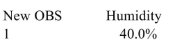Predict the ozone level for a day when the relative humidity is 40%.

The following MINITAB output presents a multiple regression equatior $\hat { y }$ =b₀+b₁x₁+b₂x₂+b₃x₃+b₄x₄ The regression equation is $\mathrm { Y } = 5.5079 + 1.6552 \mathrm { X } 1 - 1.1088 \mathrm { X } 2 + 1.3981 \mathrm { X } 3 - 1.2465 \mathrm { X } 4$ Predictor Coef SE Coef T P Constant 5.5079 0.7640 1.1002 0.314 X1 1.6552 0.7032 3.1929 0.002 X2 -1.1088 0.6023 -3.2310 0.005 X3 1.3981 0.8970 1.8137 0.087 X4 -1.2465 0.8251 -1.1433 0.354 $\text { Analysis of Variance }$ Source DF SS MS F P Regression 4 637.5 159.4 7.1480 0.003 Residual Error 40 893.2 22.3 Total 44 1,530.7 Let $\beta _ { 1 }$ be the coefficient $X _ { 1 }$ Test the hypothesis $H _ { 0 } : \beta _ { 1 } = 0$ rersus $H _ { 1 } : \beta _ { 1 } \neq 0 \text { at the } \alpha = 0.05$ level. What do you conclude?

Use the given set of points to a). Compute b₁. b). Compute the residual standard deviation s_e. c). Compute the sum of squares for x, $\sum ( x - \bar { x } ) ^ { 2 }$ d). Compute the standard error of b₁, s_b. e). Find the critical value for a 95% confidence interval for $\beta_1$ f). Compute the margin of error for a 95% confidence interval for $\beta_1$ g). Construct a 95% confidence interval for $\beta _ { 1 }$ h). Test the null hypothesis $H _ { 0 } : \beta _ { 1 } = 0$ versus $H _ { 1 } : \beta _ { 1 } \neq 0$ Use the $a$ =0.05 level of significance. x 8 11 15 13 6 8 12 13 y 23 27 37 33 17 20 29 36