Exam 4: Summarizing Bivariate Data
Exam 1: Basic Ideas39 Questions
Exam 2: Graphical Summaries of Data40 Questions
Exam 3: Numerical Summaries of Data76 Questions
Exam 4: Summarizing Bivariate Data33 Questions
Exam 5: Probability99 Questions
Exam 6: Discrete Probability Distributions76 Questions
Exam 7: The Normal Distribution131 Questions
Exam 8: Confidence Intervals62 Questions
Exam 9: Hypothesis Testing115 Questions
Exam 10: Two-Sample Confidence Intervals44 Questions
Exam 11: Two-Sample Hypothesis Tests43 Questions
Exam 12: Tests With Qualitative Data26 Questions
Exam 13: Inference in Linear Models51 Questions
Exam 14: Analysis of Variance48 Questions
Exam 15: Nonparametric Statistics27 Questions
Select questions type
The following display from a graphing calculator presents the least-squares regression line for predicting the price of a certain commodity (y) from the price of a barrel of oil (x). 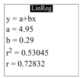 Predict the commodity price when oil costs $107 per barrel.
Free
(Multiple Choice)
4.8/5  (51)
(51)
Correct Answer: Verified
D
The following MINITAB output presents the least squares regression line for predicting the price of a certain commodity from the price of a barrel of oil.
The regression equation is
Predictor Coef SE Coef Constant 30.483819 33.659605 0.90565 0.416341 Oil 1.633495 0.33602 4.861308 0.008272
Write the equation of the least-squares regression line.
Free
(Multiple Choice)
4.9/5 (41)
Correct Answer:Verified
A
As with many other construction materials, the price of gravel (per ton) depends on the quantity of material ordered. The following table presents the unit cost (dollars/ton) for gravel for various order sizes (in tons).
Tons of Gravel Unit Cost(dollars/ton) 10 29.60 20 22.06 30 19.88 40 19.05 50 17.84 60 16.93 70 17.86 80 17.36 90 16.74
Which of the following graphs is the correct residual plot for the data set? (Hint: create your own residual plot
And compare it to those shown below.)
Free
(Multiple Choice)
4.8/5 (36)
Correct Answer:Verified
B
An automotive engineer computed a least-squares regression line for predicting the gas mileage (mile per gallon) of a certain vehicle from its speed in mph. The results are presented in the Following Excel output.
Coefficients Intercept 38.3949789 Speed -0.18832886
Write the equation of the least-squares regression line.
(Multiple Choice)
4.8/5 (37)
The following table presents the number of police officers (per 100,000 citizens) and the annual murder rate (per 100,000 citizens) for a sample of cities. Police Officers (per 100,000) Murders (per 100,000 per yr) 1377 32 1324 38 1068 47 1443 33 1289 42 1206 39 Construct a scatter plot of the per capita murder rate (y) versus the per capita number of police officers(x))
(Multiple Choice)
5.0/5 (31)
One of the primary feeds for beef cattle is corn. The following table presents the average price in dollars for a bushel of corn and a pound of ribeye steak for 10 consecutive months. Corn Price ( \/ bu) Ribeye Price (\ /) 6.02 12.71 6.48 13.07 5.77 12.00 5.95 12.48 5.99 12.36 6.55 14.17
The least-squares regression line for predicting the ribeye price from the corn price is Predict the ribeye price in a month when the corn price was $6.28 per bushel.
(Multiple Choice)
4.8/5 (46)
The following table presents the average price in dollars for a dozen eggs and a gallon of milk in several recent years.
Dozen eggs Gallon of milk 1.89 3.53 1.81 3.56 1.84 3.48 1.77 3.57 1.65 3.50 1.82 3.60 1.63 3.47 1.63 3.41
The least-squares regression equation is . If the price of eggs differs by $0.25 From one year to the next, by how much would you expect the price of milk to differ?
(Multiple Choice)
4.8/5 (32)
Of points 1, 2, and 3 shown below, which is the most influential? 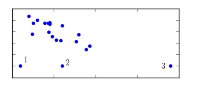
(Multiple Choice)
4.8/5 (43)
Compute the least-squares regression line for predicting y from x given the following summary statistics:
=7.4 =2.9 =47.1 =8.6 r=0.84
(Multiple Choice)
4.9/5 (39)
A blood pressure measurement consists of two numbers: the systolic pressure, which is the maximum pressure taken when the heart is contracting, and the diastolic pressure, which is the Minimum pressure taken at the beginning of the heartbeat. Blood pressures were measured, in Millimeters of mercury (mmHg), for a sample of eight adults. The following table presents the
Results.
Systolic Diastolic 127 92 125 94 135 87 110 75 123 89 121 87 118 87 127 93
The least-squares regression equation is . If the systolic pressures of two patients Differ by 8 mmHg, by how much would you predict their diastolic pressures to differ?
(Multiple Choice)
4.9/5 (32)
One of the primary feeds for beef cattle is corn. The following table presents the average price in dollars for a bushel of corn and a pound of ribeye steak for 10 consecutive months. Corn Price (\ / bu ) Ribeye Price (\ /1b) 6.25 13.75 6.20 12.86 5.85 12.61 5.74 12.66 6.44 13.94 5.81 12.75 5.97 12.66 6.59 14.25 5.72 12.87 6.56 14.11
The correlation coefficient between the corn price and the ribeye price is 0.918. Which of the Following is the best interpretation of the correlation coefficient?
(Multiple Choice)
4.8/5 (41)
The following display from a graphing calculator presents the least-squares regression line for predicting the price of a certain commodity (y) from the price of a barrel of oil (x). 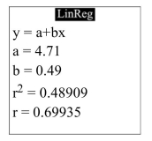 Write the equation of the least-squares regression line.
(Multiple Choice)
4.8/5 (40)
The following table shows the per-person carbon dioxide emissions for the United States and for the rest of the world over six years.
Non-U.S. U.S. 4.2 18 3.8 17.5 4 17 3 18.6 3.9 17.5 3.8 16.5
The least-squares regression equation is . If the non-U.S. emissions differ by 0.5 From one year to the next, by how much would you predict the U.S. emissions to differ?
(Multiple Choice)
4.9/5 (37)
For the following data set, compute the coefficient of determination.
x 8 6 3 2 10 4 y 21 24 20 33 27 27
(Multiple Choice)
4.8/5 (48)
The following table lists the heights in inches and weights in pounds of six football quarterbacks.
Height Weight 72 217 71 205 76 215 75 212 71 219 76 221
The least-squares regression equation is . If two quarterbacks differ in height by 6 inches, by how much would you predict their weights to differ?
(Multiple Choice)
4.9/5 (40)
As with many other construction materials, the price of gravel (per ton) depends on the quantity of material ordered. The following table presents the unit cost (dollars/ton) for gravel for various order sizes (in
Tons).
Tons of Gravel Unit Cost (dollars/ton) 73 16.49 22 21.14 89 15.98 86 16.24 60 17.34 95 16.13 56 16.71 31 20.02 90 17.05 23 21.76
Compute the coefficient of determination.
(Multiple Choice)
5.0/5 (35)
For which of the following scatter plots is the correlation coefficient an appropriate summary?
(Multiple Choice)
4.8/5 (37)
An automotive engineer computed a least-squares regression line for predicting the gas mileage (miles per gallon, or mpg) of a certain vehicle from its speed in mph. The results are presented in The following Excel output.
Coefficients Intercept 38.5176991 Speed -0.19495575
Predict the gas mileage when the vehicle is traveling at 56 mph.
(Multiple Choice)
4.9/5 (43)
The common cricket can be used as a crude thermometer. The colder the temperature, the slower the rate of chirping. The table below shows the average chirp rate of a cricket at various temperatures.
Chirp Rate (chirps/second) Temperature 1.9 47.7 2.7 67.7 2.8 65.4 1.4 42.8 1.7 54.7 3.0 63.3
The least-squares regression line for predicting the temperature from the chirp rate is Predict the temperature if the chirp rate is 1.6 chirps per second.
(Multiple Choice)
4.7/5 (36)
The following table presents the number of police officers (per 100,000 citizens) and the annual murder rate (per 100,000 citizens) for a sample of cities. Police Officers (per 100,000) Murders (per 100,000 per yr) 1252 37 1352 34 1271 41 1275 39 1472 35 1047 52 The correlation coefficient between the per capita number of police officers and the per capita murder rates -0.899. Which of the following is the best interpretation of the correlation coefficient?
(Multiple Choice)
4.8/5 (39)
Filters
- Essay(0)
- Multiple Choice(0)
- Short Answer(0)
- True False(0)
- Matching(0)