Exam 13: Inference in Linear Models

Use the given set of points to construct a 95% confidence interval for $\beta _ { 1 }$ . x 8 6 5 9 6 12 14 11 y 21 18 15 21 21 28 28 24

The following table lists values measured for 10 consecutive eruptions of the geyser Old Faithful in Yellowstone National Park. They are the duration, in minutes, of the eruption $\left( x _ { 1 } \right)$ , the dormant Period before the eruption $\left( x _ { 2 } \right)$ , and the dormant period after the eruption (y). y 3.5 80 84 4.1 84 50 2.3 50 93 4.7 93 55 1.7 55 76 4.9 76 58 1.7 58 74 4.6 74 75 3.4 75 80 4.3 80 56 Construct the multiple regression equation $\hat { y}$ =b₀+b₁x₁+b₂x₂

Use the given set of points to compute the margin of error for a 95% confidence interval for $\beta _ { 1 }$ . x 9 9 13 7 9 14 8 10 y 18 23 27 19 24 35 19 25

Use the given set of points to compute the predicted value $\hat { y }$ for the given value of x. x 13 14 16 13 13 16 y 61 66 75 60 64 72 x=12

Use the given set of points to compute b₀ and b₁. x 16 12 14 19 18 10 y 74 58 62 82 82 49 xequals12

Construct the multiple regression sequence $\hat { y }$ =b₀+b₁x₁+b₂x₂+b₃x₃ for the following data set: y 51.0 80 34 7.5 34.3 60 22 2.5 31.5 60 24 5.0 33.2 60 23 4.0 49.2 60 29 6.5 46.7 70 27 7.5 30.4 70 32 4.0 43.2 60 25 5.5 30.6 60 26 3.5 43.3 70 28 7.5

Use the given set of points to compute the sum of squares for x,(x- . x 13 13 20 16 12 20 y 55 59 89 72 56 85 x=17

In a study of reaction times, the time to respond to a visual stimulus (x) and the time to respond to an auditory stimulus (y) were recorded for each of 6 subjects. Times were measured in thousandths of A second. The results are presented in the following table. The following MINITAB output describes the fit of a linear model to these data. Assume that the ass of the linear model are satisfied. The regression equation is Auditory $= 204.285245 + 0.286943$ Visual Predictor Coef SE Coef T P Constant 204.285245 10.451581 19.54587 0.000041 Visual 0.286943 0.051998 5.518383 0.005265 What is the intercept of the least-squares regression line?

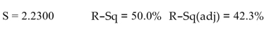
The following display from a TI-84 Plus calculator presents the results of a test of the null hypothesis 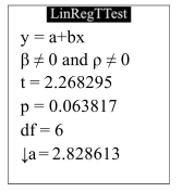$H _ { 0 } : \beta _ { 1 } = 0$ How many degrees of freedom did the calculator use?

The following MINITAB output presents a multiple regression equation $\hat { y } = b _ { 0 } + b _ { 1 } x _ { 1 } + b _ { 2 } x _ { 2 } +$ $+ b _ { 4 } x _ { 4 }$ . The regression equation is $\mathrm { Y } = 5.3535 + 0.7929 \mathrm { X } 1 - 0.8918 \mathrm { X } 2 + 0.5297 \mathrm { X } 3 - 1.7948 \mathrm { X } 4$ Predictor Coef SE Coef T P Constant 5.3535 0.7240 0.8771 0.338 X1 0.7929 0.7986 3.3073 0.002 X2 -0.8918 0.8208 -2.9354 0.009 X3 0.5297 0.8980 1.9458 0.083 X4 -1.7948 0.6461 -1.0262 0.340 $\text { Analysis of Variance }$ Source DF SS MS F P Regression 4 1,188.8 297.2 7.7396 0.003 Residual Error 31 1,190.1 38.4 Total 35 2,378.9 b₃x₃ What percentage of the variation in y is explained by the model?

The following MINITAB output presents a multiple regression equation $\hat { y } = b _ { 0 } + b _ { 1 } x _ { 1 } + b _ { 2 } x _ { 2 } + b _ { 3 } x _ { 3 }$ $+ b _ { 4 } x _ { 4 }$ . The regression equation is $\mathrm { Y } = 1.9568 + 1.7369 \mathrm { X } 1 + 1.1099 \mathrm { X } 2 - 1.2672 \mathrm { X } 3 + 1.6080 \mathrm { X } 4$ Predictor Coef SE Coef T P Constant 1.9568 0.8248 1.1277 0.345 X1 1.7369 0.7980 3.4296 0.004 X2 1.1099 0.7500 -3.2529 0.006 X3 -1.2672 0.7534 1.8730 0.076 X4 1.6080 0.8733 -0.9328 0.349 $\text { Analysis of Variance }$ Source DF SS MS F P Regression 4 503.9 126.0 5.0806 0.003 Residual Error 40 990.4 24.8 Total 44 1,494.3 Predict the value of $\mathrm { y }$ when $x _ { 1 } = 1 , x _ { 2 } = 2 , x _ { 3 } = 3 , x _ { 4 } = 6$

The following MINITAB output presents a 95% confidence interval for the mean ozone level on days when the relative humidity is 55%, and a 95% prediction interval for the ozone level on a Particular day when the relative humidity is 55%. The units of ozone are parts per billion. Predicted Values for New Observations New Obs Fit SE Fit 95.0\% CI 95.0\% PI 1 38.46 1.4 (35.72,41.20) (22.17,54.75) 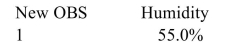What is the point estimate for the mean ozone level for days when the relative humidity is $55 \%$ ?

The summary statistics for a certain set of points are: $n = 10 , s _ { \mathrm { e } } = 3.857 , \sum ( x - \bar { x } ) ^ { 2 } = 13.030$ , and $b _ { 1 } = 1.747$ . Assume the conditions of the linear model hold. A $99 \%$ confidence interval for $\beta _ { 1 }$ will be constructed. What is the critical value?

Use the given set of points to compute the standard error of , . x 5 15 12 6 8 10 5 14 y 15 37 28 18 22 26 13 33

In a study of reaction times, the time to respond to a visual stimulus (x) and the time to respond to an auditory stimulus (y) were recorded for each of 8 subjects. Times were measured in thousandths Of a second. The results are presented in the following table. Visual Auditory 208 200 177 175 250 233 248 234 152 155 164 161 196 190 238 230 Compute the least-squares regression line for predicting auditory response time (y) from visual response Time (x).

In a study of reaction times, the time to respond to a visual stimulus (x) and the time to respond to an auditory stimulus (y) were recorded for each of 8 subjects. Times were measured in thousandths of A second. The results are presented in the following table. Visual Auditory 201 241 164 237 189 243 168 243 190 244 239 247 169 237 236 244 Construct a 99% confidence interval for the mean auditory response time for subjects with a visual Response time of 171.

The summary statistics for a certain set of points are: $n = 18 , s _ { \mathrm { e } } = 8.078 , \sum ( x - \bar { x } ) ^ { 2 } = 7.614$ , and $b _ { 1 } = 1.29$ Assume the conditions of the linear model hold. A 99% confidence interval for $\beta _ { 1 }$ will be constructed. Test the null hypothesis $H _ { 0 } : \beta _ { 1 } = 0$ versus $H _ { 0 } : \beta _ { 1 } > 0$ . Use the $\alpha = 0.01$ level of significance.

The following MINITAB output presents a multiple regression equatior $\hat { y }$ =b₀+b₁x₁+b₂x₂+b₃x₃+b₄x₄ The regression equation is $\mathrm { Y } = 2.5919 - 1.3391 \mathrm { X } 1 + 0.6212 \mathrm { X } 2 + 1.6435 \mathrm { X } 3 + 1.4269 \mathrm { X } 4$ Predictor Coef SE Coef T P Constant 2.5919 0.6269 1.1668 0.337 X1 -1.3391 0.6716 3.5190 0.002 X2 0.6212 0.8488 -3.2848 0.004 X3 1.6435 0.7934 1.8821 0.090 X4 1.4269 0.7679 -0.9879 0.345 $\text { Analysis of Variance }$ Source DF SS MS F P Regression 4 735.9 184.0 7.7311 0.003 Residual Error 25 594.6 23.8 Total 29 1,330.5 Let $\beta _ { 3 }$ be the coefficient $X _ { 3 }$ Test the hypothesis $H _ { 0 } : \beta _ { 3 } = 0$ versus $H _ { 1 } : \beta _ { 3 } \neq 0 \text { at the } \alpha = 0.05$ level. What do you conclude?

Use the given set of points to compute the residual standard deviation $s _ { \mathrm { e } }$ x 13 10 10 11 13 7 11 6 y 32 26 23 24 28 16 26 21

In a study of reaction times, the time to respond to a visual stimulus (x) and the time to respond to an auditory stimulus (y) were recorded for each of 6 subjects. Times were measured in thousandths of A second. The results are presented in the following table. The following MINITAB output describes the fit of a linear model to these data. Assume that the assumptions Of the linear model are satisfied. The regression equation is Auditory $= 212.498779 + 0.245553$ Visual Predictor Coef SE Coef T P Constant 212.498779 26.573957 7.996505 0.001327 Visual 0.245553 0.124489 1.972495 0.119828 Can you conclude that the response time to visual stimulus is useful in predicting the response time for Auditory stimulus? Answer this question using the α = 0.05 level of significance.