Exam 13: Simple Linear Regression

TABLE 13-2 A candy bar manufacturer is interested in trying to estimate how sales are influenced by the price of their product. To do this, the company randomly chooses 6 small cities and offers the candy bar at different prices. Using candy bar sales as the dependent variable, the company will conduct a simple linear regression on the data below: River Falls 1.30 100 Hudson 1.60 90 Ellsworth 1.80 90 Prescott 2.00 40 Rock Elm 2.40 38 Stillwater 2.90 32 -Referring to Table 13-2, what is the estimated slope for the candy bar price and sales data?

TABLE 13-11 A computer software developer would like to use the number of downloads (in thousands) for the trial version of his new shareware to predict the amount of revenue (in thousands of dollars) he can make on the full version of the new shareware. Following is the output from a simple linear regression along with the residual plot and normal probability plot obtained from a data set of 30 different sharewares that he has developed: Regression Statistics Multiple R 0.8691 R Square 0.7554 Adjusted R Square 0.7467 Standard Error 44.4765 Observations 30.0000 $\text { ANOVA }$ df SS MS F Significance F Regression 1 171062.9193 171062.9193 86.4759 0.0000 Residual 28 55388.4309 1978.1582 Total 29 226451.3503 Coefficients Standard Error t Stat P-value Lower 95\% \multicolumn 1 r Upper 95\% Intercept -95.0614 26.9183 -3.5315 0.0015 -150.2009 -39.9218 Download 3.7297 0.4011 9.2992 0.0000 2.9082 4.5513 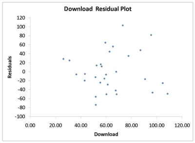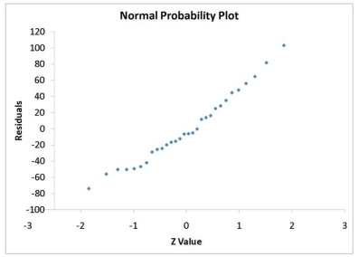-Referring to Table 13-11, the Durbin-Watson statistic is inappropriate for this data set.

TABLE 13-3 The director of cooperative education at a state college wants to examine the effect of cooperative education job experience on marketability in the work place. She takes a random sample of 4 students. For these 4, she finds out how many times each had a cooperative education job and how many job offers they received upon graduation. These data are presented in the table below. Student CoopJobs JobOffer 1 1 4 2 2 6 3 1 3 4 0 1 -Referring to Table 13-3, suppose the director of cooperative education wants to construct a 95% prediction interval for the number of job offers received by a student who has had exactly two cooperative education jobs. The t critical value she would use is ________.

TABLE 13-12 The manager of the purchasing department of a large saving and loan organization would like to develop a model to predict the amount of time (measured in hours) it takes to record a loan application. Data are collected from a sample of 30 days, and the number of applications recorded and completion time in hours is recorded. Below is the regression output: Regression Statistics Multiple R 0.9447 R Square 0.8924 Adjusted R 0.8886 Square Standard 0.3342 Error Observations 30 $\text { ANOVA }$ df SS MS F Significance F Regression 1 25.9438 25.9438 232.2200 4.3946-15 Residual 28 3.1282 0.1117 Total 29 29.072 Coefficients Standard Error t Stat P -value Lower 95\% Upper 95\% Intercept 0.4024 0.1236 3.2559 0.0030 0.1492 0.6555 Applications Recorded 0.0126 0.0008 15.2388 4.3946-15 0.0109 0.0143 Note: 4.3946E-15 is 4.3946*10^-15 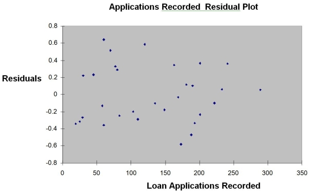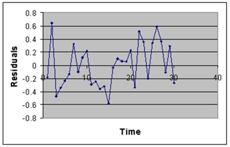-Referring to Table 13-12, there is sufficient evidence that the amount of time needed linearly depends on the number of loan applications at a 5% level of significance.

TABLE 13-4 The managers of a brokerage firm are interested in finding out if the number of new clients a broker brings into the firm affects the sales generated by the broker. They sample 12 brokers and determine the number of new clients they have enrolled in the last year and their sales amounts in thousands of dollars. These data are presented in the table that follows. 1 27 52 2 11 37 3 42 64 4 33 55 5 15 29 6 15 34 7 25 58 8 36 59 9 28 44 10 30 48 11 17 31 12 22 38 -Referring to Table 13-4, the managers of the brokerage firm wanted to test the hypothesis that the population slope was equal to 0. For a test with a level of significance of 0.01, the null hypothesis should be rejected if the value of the test statistic is ________.

TABLE 13-3 The director of cooperative education at a state college wants to examine the effect of cooperative education job experience on marketability in the work place. She takes a random sample of 4 students. For these 4, she finds out how many times each had a cooperative education job and how many job offers they received upon graduation. These data are presented in the table below. Student CoopJobs JobOffer 1 1 4 2 2 6 3 1 3 4 0 1 -Referring to Table 13-3, the director of cooperative education wanted to test the hypothesis that the population slope was equal to 3.0. The value of the test statistic is ________.

TABLE 13-3 The director of cooperative education at a state college wants to examine the effect of cooperative education job experience on marketability in the work place. She takes a random sample of 4 students. For these 4, she finds out how many times each had a cooperative education job and how many job offers they received upon graduation. These data are presented in the table below. Student CoopJobs JobOffer 1 1 4 2 2 6 3 1 3 4 0 1 -Referring to Table 13-3, set up a scatter plot.

The width of the prediction interval for the predicted value of Y is dependent on

TABLE 13-3 The director of cooperative education at a state college wants to examine the effect of cooperative education job experience on marketability in the work place. She takes a random sample of 4 students. For these 4, she finds out how many times each had a cooperative education job and how many job offers they received upon graduation. These data are presented in the table below. Student CoopJobs JobOffer 1 1 4 2 2 6 3 1 3 4 0 1 -Referring to Table 13-3, suppose the director of cooperative education wants to construct both a 95% confidence interval estimate and a 95% prediction interval for X = 2. The confidence interval estimate would be the wider of the two intervals.

TABLE 13-13 In this era of tough economic conditions, voters increasingly ask the question: "Is the educational achievement level of students dependent on the amount of money the state in which they reside spends on education?" The partial computer output below is the result of using spending per student ($) as the independent variable and composite score which is the sum of the math, science and reading scores as the dependent variable on 35 states that participated in a study. The table includes only partial results. Regression Statistics Multiple R 0.3122 R Square 0.0975 Adjusted R 0.0701 Square Standard 26.9122 Error Observations 35 $\text { ANOVA }$ df SS MS F Regression 1 2581.5759 Residual 724.2674 Total 34 26482.4000 Coefficients Standard Error t Stat P-value Intercept 595.540251 22.115176 Spending per Student () 0.007996 0.004235 -Referring to Table 13-13, the decision on the test of whether spending per student affects composite score using a 5% level of significance is to ________ (reject or not reject)H₀.

TABLE 13-3 The director of cooperative education at a state college wants to examine the effect of cooperative education job experience on marketability in the work place. She takes a random sample of 4 students. For these 4, she finds out how many times each had a cooperative education job and how many job offers they received upon graduation. These data are presented in the table below. Student CoopJobs JobOffer 1 1 4 2 2 6 3 1 3 4 0 1 -Referring to Table 13-3, the coefficient of determination is ________.

TABLE 13-7 An investment specialist claims that if one holds a portfolio that moves in the opposite direction to the market index like the S&P 500, then it is possible to reduce the variability of the portfolio's return. In other words, one can create a portfolio with positive returns but less exposure to risk. A sample of 26 years of S&P 500 index and a portfolio consisting of stocks of private prisons, which are believed to be negatively related to the S&P 500 index, is collected. A regression analysis was performed by regressing the returns of the prison stocks portfolio (Y) on the returns of S&P 500 index (X) to prove that the prison stocks portfolio is negatively related to the S&P 500 index at a 5% level of significance. The results are given in the following Excel output. Coefficients Standard Error T Stat p -value Intercept 4.8660 0.3574 13.6136 8.7932-13 S \&P -0.5025 0.0716 -7.0186 2.94942-07 Note: 2.94942E-07 = 2.94942*10⁻⁷ -Referring to Table 13-7, to test whether the prison stocks portfolio is negatively related to the S&P 500 index, the p-value of the associated test statistic is

TABLE 13-1 A large national bank charges local companies for using their services. A bank official reported the results of a regression analysis designed to predict the bank's charges (Y)measured in dollars per month11ed1eb9_2726_0788_bd82_e76f79f37173_TB1604_00for services rendered to local companies. One independent variable used to predict service charges to a company is the company's sales revenue (X)11ed1eb9_2726_0788_bd82_e76f79f37173_TB1604_00measured in millions of dollars. Data for 21 companies who use the bank's services were used to fit the model: Yᵢ = β₀ + β₁Xi + Eᵢ The results of the simple linear regression are provided below. $Y = - 2,700 + 20 X , S Y X = 65 \text {, two-tail } p \text {-value } = 0.034 \text { (for testing } \beta _ { 1 } \text { ) }$ -Referring to Table 13-1, interpret the estimate of β₀, the Y-intercept of the line.

TABLE 13-5 The managing partner of an advertising agency believes that his company's sales are related to the industry sales. He uses Microsoft Excel to analyze the last 4 years of quarterly data (i.e., n = 16) with the following results: Regression Statistics Multiple R 0.802 R Square 0.643 Adjusted R Square 0.618 Standard Error SYX 0.9224 Observations 16 ANOVA df SS MS F Sig.F Regression 1 21.497 21.497 25.27 0.000 Error 14 11.912 0.851 Total 15 33.409 p -value Intercept 3.962 1.440 2.75 0.016 Industry 0.040451 0.008048 5.03 0.000 Durbin-Watson Statistic $1.59$ -Referring to Table 13-5, the standard error of the estimate is ________.

TABLE 13-4 The managers of a brokerage firm are interested in finding out if the number of new clients a broker brings into the firm affects the sales generated by the broker. They sample 12 brokers and determine the number of new clients they have enrolled in the last year and their sales amounts in thousands of dollars. These data are presented in the table that follows. 1 27 52 2 11 37 3 42 64 4 33 55 5 15 29 6 15 34 7 25 58 8 36 59 9 28 44 10 30 48 11 17 31 12 22 38 -Referring to Table 13-4, suppose the managers of the brokerage firm want to construct n a 99% prediction interval for the sales made by a broker who has brought into the firm 18 new clients. The t critical value they would use is ________.

TABLE 13-5 The managing partner of an advertising agency believes that his company's sales are related to the industry sales. He uses Microsoft Excel to analyze the last 4 years of quarterly data (i.e., n = 16) with the following results: Regression Statistics Multiple R 0.802 R Square 0.643 Adjusted R Square 0.618 Standard Error SYX 0.9224 Observations 16 ANOVA df SS MS F Sig.F Regression 1 21.497 21.497 25.27 0.000 Error 14 11.912 0.851 Total 15 33.409 p -value Intercept 3.962 1.440 2.75 0.016 Industry 0.040451 0.008048 5.03 0.000 Durbin-Watson Statistic $1.59$ -Referring to Table 13-5, the coefficient of determination is ________.

TABLE 13-2 A candy bar manufacturer is interested in trying to estimate how sales are influenced by the price of their product. To do this, the company randomly chooses 6 small cities and offers the candy bar at different prices. Using candy bar sales as the dependent variable, the company will conduct a simple linear regression on the data below: River Falls 1.30 100 Hudson 1.60 90 Ellsworth 1.80 90 Prescott 2.00 40 Rock Elm 2.40 38 Stillwater 2.90 32 -Referring to Table 13-2, if the price of the candy bar is set at $2, the predicted sales will be

The confidence interval for the mean of Y is always narrower than the prediction interval for an individual response Y given the same data set, X value, and confidence level.

TABLE 13-2 A candy bar manufacturer is interested in trying to estimate how sales are influenced by the price of their product. To do this, the company randomly chooses 6 small cities and offers the candy bar at different prices. Using candy bar sales as the dependent variable, the company will conduct a simple linear regression on the data below: River Falls 1.30 100 Hudson 1.60 90 Ellsworth 1.80 90 Prescott 2.00 40 Rock Elm 2.40 38 Stillwater 2.90 32 -Referring to Table 13-2, if the price of the candy bar is set at $2, the estimated mean sales will be

TABLE 13-3 The director of cooperative education at a state college wants to examine the effect of cooperative education job experience on marketability in the work place. She takes a random sample of 4 students. For these 4, she finds out how many times each had a cooperative education job and how many job offers they received upon graduation. These data are presented in the table below. Student CoopJobs JobOffer 1 1 4 2 2 6 3 1 3 4 0 1 -Referring to Table 13-3, suppose the director of cooperative education wants to construct a 95% prediction interval estimate for the number of job offers received by students who have had exactly one cooperative education job. The prediction interval is from ________ to ________.