Exam 14: Introduction to Multiple Regression

TABLE 14-18 A logistic regression model was estimated in order to predict the probability that a randomly chosen university or college would be a private university using information on mean total Scholastic Aptitude Test score (SAT) at the university or college, the room and board expense measured in thousands of dollars (Room/Brd), and whether the TOEFL criterion is at least 550 (Toefl550 = 1 if yes, 0 otherwise.) The dependent variable, Y, is school type (Type = 1 if private and 0 otherwise). The Minitab output is given below: Logistic Regression Table Odds 95\% Predictor Coef SE Coef Ratio Lower Upper Constant -27.118 6.696 -4.05 0.000 SAT 0.015 0.004666 3.17 0.002 1.01 1.01 1.02 Toefl550 -0.390 0.9538 -0.41 0.682 0.68 0.10 4.39 Room/Brd 2.078 0.5076 4.09 0.000 7.99 2.95 21.60 Log-Likelihood $= - 21.883$ Test that all slopes are zero: $\mathrm { G } = 62.083 , \mathrm { DF } = 3 , p$ -value $= 0.000$ Goodness-of-Fit Tests Method Chi-Square DF P Pearson 143.551 76 0.000 Deviance 43.767 76 0.999 Hosmer-Lemeshow 15.731 8 0.046 -Referring to Table 14-18, there is not enough evidence to conclude that SAT score makes a significant contribution to the model in the presence of the other independent variables at a 0.05 level of significance.

TABLE 14-18 A logistic regression model was estimated in order to predict the probability that a randomly chosen university or college would be a private university using information on mean total Scholastic Aptitude Test score (SAT) at the university or college, the room and board expense measured in thousands of dollars (Room/Brd), and whether the TOEFL criterion is at least 550 (Toefl550 = 1 if yes, 0 otherwise.) The dependent variable, Y, is school type (Type = 1 if private and 0 otherwise). The Minitab output is given below: Logistic Regression Table Odds 95\% Predictor Coef SE Coef Ratio Lower Upper Constant -27.118 6.696 -4.05 0.000 SAT 0.015 0.004666 3.17 0.002 1.01 1.01 1.02 Toefl550 -0.390 0.9538 -0.41 0.682 0.68 0.10 4.39 Room/Brd 2.078 0.5076 4.09 0.000 7.99 2.95 21.60 Log-Likelihood $= - 21.883$ Test that all slopes are zero: $\mathrm { G } = 62.083 , \mathrm { DF } = 3 , p$ -value $= 0.000$ Goodness-of-Fit Tests Method Chi-Square DF P Pearson 143.551 76 0.000 Deviance 43.767 76 0.999 Hosmer-Lemeshow 15.731 8 0.046 -Referring to Table 14-18, what is the p-value of the test statistic when testing whether the model is a good-fitting model?

TABLE 14-3 An economist is interested to see how consumption for an economy (in $ billions) is influenced by gross domestic product ($ billions) and aggregate price (consumer price index). The Microsoft Excel output of this regression is partially reproduced below. SUMMARY OUTPUT Regression Statistics Multiple R 0.991 R Square 0.982 Adjusted R Square 0.976 Standard Error 0.299 Observations 10 ANOVA df SS MS F Signif F Regression 2 33.4163 16.7082 186.325 0.0001 Residual 7 0.6277 0.0897 Total 9 34.0440 Coeff StdError t Stat p -value Intercept -0.0861 0.5674 -0.152 0.8837 GDP 0.7654 0.0574 13.340 0.0001 Price -0.0006 0.0028 -0.219 0.8330 -Referring to Table 14-3, the p-value for GDP is

TABLE 14-17 Given below are results from the regression analysis where the dependent variable is the number of weeks a worker is unemployed due to a layoff (Unemploy) and the independent variables are the age of the worker (Age), the number of years of education received (Edu), the number of years at the previous job (Job Yr), a dummy variable for marital status (Married: 1 = married, 0 = otherwise), a dummy variable for head of household (Head: 1 = yes, 0 = no) and a dummy variable for management position (Manager: 1 = yes, 0 = no). We shall call this Model 1. The coefficients of partial determination ( 2 Yj. (Allvariables except $j$ ) ) of each of the 6 predictors are, respectively, 0.2807, 0.0386, 0.0317, 0.0141, 0.0958, and 0.1201. Regression Statistics Multiple R 0.7035 R Square 0.4949 Adjusted R 0.4030 Square Standard 18.4861 Error 40 Observations $\text { ANOVA }$ df SS MS F significance F Regression 6 11048.6415 1841.4402 5.3885 0.00057 Residual 33 11277.2586 341.7351 Total 39 22325.9 Coefficients Standard Error t Stat P-value Lower 95\% Upper 95\% Intercept 32.6595 23.18302 1.4088 0.1683 -14.5067 79.8257 Age 1.2915 0.3599 3.5883 0.0011 0.5592 2.0238 Edu -1.3537 1.1766 -1.1504 0.2582 -3.7476 1.0402 Job Yr 0.6171 0.5940 1.0389 0.3064 -0.5914 1.8257 Married -5.2189 7.6068 -0.6861 0.4974 -20.6950 10.2571 Head -14.2978 7.6479 -1.8695 0.0704 -29.8575 1.2618 Manager -24.8203 11.6932 -2.1226 0.0414 -48.6102 -1.0303 Model 2 is the regression analysis where the dependent variable is Unemploy and the independent variables are Age and Manager. The results of the regression analysis are given below: Regression Statistics Multiple R 0.6391 R Square 0.4085 Adjusted R 0.3765 Square Standard Error 18.8929 Observations 40 $\text { ANOVA }$ df SS MS F Significance F Regression 2 9119.0897 4559.5448 12.7740 0.0000 Residual 37 13206.8103 356.9408 Total 39 22325.9 Coefficients Standard Error t Stat P -value Intercept -0.2143 11.5796 -0.0185 0.9853 Age 1.4448 0.3160 4.5717 0.0000 Manager -22.5761 11.3488 -1.9893 0.0541 -Referring to Table 14-17 Model 1, ________ of the variation in the number of weeks a worker is unemployed due to a layoff can be explained by the marital status while controlling for the other independent variables.

TABLE 14-8 A financial analyst wanted to examine the relationship between salary (in $1,000) and 4 variables: age (X₁ = Age), experience in the field (X₂ = Exper), number of degrees (X₃ = Degrees), and number of previous jobs in the field (X₄ = Prevjobs). He took a sample of 20 employees and obtained the following Microsoft Excel output: SUMMARY OUTPUT Regression Statistics Multiple R 0.992 R Square 0.984 Adjusted R Square 0.979 Standard Error 2.26743 Observations 20 ANOVA df SS MS F Signif F Regression 4 4609.83164 1152.45791 224.160 0.0001 Residual 15 77.11836 5.14122 Total 19 4686.95000 Coeff StdError t Stat p -value Intercept -9.611198 2.77988638 -3.457 0.0035 Age 1.327695 0.11491930 11.553 0.0001 Exper -0.106705 0.14265559 -0.748 0.4660 Degrees 7.311332 0.80324187 9.102 0.0001 Prevjobs -0.504168 0.44771573 -1.126 0.2778 -Referring to Table 14-8, the p-value of the F test for the significance of the entire regression is ________.

TABLE 14-19 The marketing manager for a nationally franchised lawn service company would like to study the characteristics that differentiate home owners who do and do not have a lawn service. A random sample of 30 home owners located in a suburban area near a large city was selected; 15 did not have a lawn service (code 0) and 15 had a lawn service (code 1). Additional information available concerning these 30 home owners includes family income (Income, in thousands of dollars), lawn size (Lawn Size, in thousands of square feet), attitude toward outdoor recreational activities (Atitude 0 = unfavorable, 1 = favorable), number of teenagers in the household (Teenager), and age of the head of the household (Age). The Minitab output is given below: Logistic Regression Table Odds 95\% CI Predictor Coef SE Coef Z P Ratio Lower Upper Constant -70.49 47.22 -1.49 0.135 Income 0.2868 0.1523 1.88 0.060 1.33 0.99 1.80 LawnSiz 1.0647 0.7472 1.42 0.154 2.90 0.67 12.54 Attitude -12.744 9.455 -1.35 0.178 0.00 0.00 326.06 Teenager -0.200 1.061 -0.19 0.850 0.82 0.10 6.56 Age 1.0792 0.8783 1.23 0.219 2.94 0.53 16.45 Log-Likelihood $= - 4.890$ Test that all slopes are zero: $\mathrm { G } = 31.808 , \mathrm { DF } = 5 , p$ -value $= 0.000$ Goodness-of-Fit Tests Method Chi-Square DF Pearson 9.313 24 0.997 Deviance 9.780 24 0.995 Hosmer-Lemeshow 0.571 8 1.000 -Referring to Table 14-19, what is the p-value of the test statistic when testing whether Attitude makes a significant contribution to the model in the presence of the other independent variables?

TABLE 14-19 The marketing manager for a nationally franchised lawn service company would like to study the characteristics that differentiate home owners who do and do not have a lawn service. A random sample of 30 home owners located in a suburban area near a large city was selected; 15 did not have a lawn service (code 0) and 15 had a lawn service (code 1). Additional information available concerning these 30 home owners includes family income (Income, in thousands of dollars), lawn size (Lawn Size, in thousands of square feet), attitude toward outdoor recreational activities (Atitude 0 = unfavorable, 1 = favorable), number of teenagers in the household (Teenager), and age of the head of the household (Age). The Minitab output is given below: Logistic Regression Table Odds 95\% CI Predictor Coef SE Coef Z P Ratio Lower Upper Constant -70.49 47.22 -1.49 0.135 Income 0.2868 0.1523 1.88 0.060 1.33 0.99 1.80 LawnSiz 1.0647 0.7472 1.42 0.154 2.90 0.67 12.54 Attitude -12.744 9.455 -1.35 0.178 0.00 0.00 326.06 Teenager -0.200 1.061 -0.19 0.850 0.82 0.10 6.56 Age 1.0792 0.8783 1.23 0.219 2.94 0.53 16.45 Log-Likelihood $= - 4.890$ Test that all slopes are zero: $\mathrm { G } = 31.808 , \mathrm { DF } = 5 , p$ -value $= 0.000$ Goodness-of-Fit Tests Method Chi-Square DF Pearson 9.313 24 0.997 Deviance 9.780 24 0.995 Hosmer-Lemeshow 0.571 8 1.000 -Referring to Table 14-19, what should be the decision ('reject' or 'do not reject')on the null hypothesis when testing whether Age makes a significant contribution to the model in the presence of the other independent variables at a 0.05 level of significance?

TABLE 14-17 Given below are results from the regression analysis where the dependent variable is the number of weeks a worker is unemployed due to a layoff (Unemploy) and the independent variables are the age of the worker (Age), the number of years of education received (Edu), the number of years at the previous job (Job Yr), a dummy variable for marital status (Married: 1 = married, 0 = otherwise), a dummy variable for head of household (Head: 1 = yes, 0 = no) and a dummy variable for management position (Manager: 1 = yes, 0 = no). We shall call this Model 1. The coefficients of partial determination ( 2 Yj. (Allvariables except $j$ ) ) of each of the 6 predictors are, respectively, 0.2807, 0.0386, 0.0317, 0.0141, 0.0958, and 0.1201. Regression Statistics Multiple R 0.7035 R Square 0.4949 Adjusted R 0.4030 Square Standard 18.4861 Error 40 Observations $\text { ANOVA }$ df SS MS F significance F Regression 6 11048.6415 1841.4402 5.3885 0.00057 Residual 33 11277.2586 341.7351 Total 39 22325.9 Coefficients Standard Error t Stat P-value Lower 95\% Upper 95\% Intercept 32.6595 23.18302 1.4088 0.1683 -14.5067 79.8257 Age 1.2915 0.3599 3.5883 0.0011 0.5592 2.0238 Edu -1.3537 1.1766 -1.1504 0.2582 -3.7476 1.0402 Job Yr 0.6171 0.5940 1.0389 0.3064 -0.5914 1.8257 Married -5.2189 7.6068 -0.6861 0.4974 -20.6950 10.2571 Head -14.2978 7.6479 -1.8695 0.0704 -29.8575 1.2618 Manager -24.8203 11.6932 -2.1226 0.0414 -48.6102 -1.0303 Model 2 is the regression analysis where the dependent variable is Unemploy and the independent variables are Age and Manager. The results of the regression analysis are given below: Regression Statistics Multiple R 0.6391 R Square 0.4085 Adjusted R 0.3765 Square Standard Error 18.8929 Observations 40 $\text { ANOVA }$ df SS MS F Significance F Regression 2 9119.0897 4559.5448 12.7740 0.0000 Residual 37 13206.8103 356.9408 Total 39 22325.9 Coefficients Standard Error t Stat P -value Intercept -0.2143 11.5796 -0.0185 0.9853 Age 1.4448 0.3160 4.5717 0.0000 Manager -22.5761 11.3488 -1.9893 0.0541 -Referring to Table 14-17 Model 1, which of the following is the correct alternative hypothesis to determine whether there is a significant relationship between percentage of students passing the proficiency test and the entire set of explanatory variables?

TABLE 14-3 An economist is interested to see how consumption for an economy (in $ billions) is influenced by gross domestic product ($ billions) and aggregate price (consumer price index). The Microsoft Excel output of this regression is partially reproduced below. SUMMARY OUTPUT Regression Statistics Multiple R 0.991 R Square 0.982 Adjusted R Square 0.976 Standard Error 0.299 Observations 10 ANOVA df SS MS F Signif F Regression 2 33.4163 16.7082 186.325 0.0001 Residual 7 0.6277 0.0897 Total 9 34.0440 Coeff StdError t Stat p -value Intercept -0.0861 0.5674 -0.152 0.8837 GDP 0.7654 0.0574 13.340 0.0001 Price -0.0006 0.0028 -0.219 0.8330 -Referring to Table 14-3, one economy in the sample had an aggregate consumption level of $4 billion, a GDP of $6 billion, and an aggregate price level of 200. What is the residual for this data point?

TABLE 14-10 You worked as an intern at We Always Win Car Insurance Company last summer. You notice that individual car insurance premiums depend very much on the age of the individual, the number of traffic tickets received by the individual, and the population density of the city in which the individual lives. You performed a regression analysis in Excel and obtained the following information: $\text { Regression Analysis }$ Regression Statistics Multiple R 0.63 R Square 0.40 Adjusted R Square 0.23 Standard Error 50.00 Observations 15.00 $\text { ANOVA }$ df SS MS F Significance F Regression 3 5994.24 2.40 0.12 Residual 11 27496.82 Total 45479.54 Coefficients Standard Error t Stat P-value Lower 99.0\% Upper 99.0\% Intercept 123.80 48.71 2.54 0.03 -27.47 275.07 AGE -0.82 0.87 -0.95 0.36 -3.51 1.87 TICKETS 21.25 10.66 1.99 0.07 -11.86 54.37 DENSITY -3.14 6.46 -0.49 0.64 -23.19 16.91 -Referring to Table 14-10, the estimated mean change in insurance premiums for every ?2 additional tickets received is ________.

TABLE 14-19 The marketing manager for a nationally franchised lawn service company would like to study the characteristics that differentiate home owners who do and do not have a lawn service. A random sample of 30 home owners located in a suburban area near a large city was selected; 15 did not have a lawn service (code 0) and 15 had a lawn service (code 1). Additional information available concerning these 30 home owners includes family income (Income, in thousands of dollars), lawn size (Lawn Size, in thousands of square feet), attitude toward outdoor recreational activities (Atitude 0 = unfavorable, 1 = favorable), number of teenagers in the household (Teenager), and age of the head of the household (Age). The Minitab output is given below: Logistic Regression Table Odds 95\% CI Predictor Coef SE Coef Z P Ratio Lower Upper Constant -70.49 47.22 -1.49 0.135 Income 0.2868 0.1523 1.88 0.060 1.33 0.99 1.80 LawnSiz 1.0647 0.7472 1.42 0.154 2.90 0.67 12.54 Attitude -12.744 9.455 -1.35 0.178 0.00 0.00 326.06 Teenager -0.200 1.061 -0.19 0.850 0.82 0.10 6.56 Age 1.0792 0.8783 1.23 0.219 2.94 0.53 16.45 Log-Likelihood $= - 4.890$ Test that all slopes are zero: $\mathrm { G } = 31.808 , \mathrm { DF } = 5 , p$ -value $= 0.000$ Goodness-of-Fit Tests Method Chi-Square DF Pearson 9.313 24 0.997 Deviance 9.780 24 0.995 Hosmer-Lemeshow 0.571 8 1.000 -Referring to Table 14-19, what are the degrees of freedom for the chi-square distribution when testing whether the model is a good-fitting model?

You have just computed a regression model in which the value of coefficient of multiple determination is 0.57. To determine if this indicates that the independent variables explain a significant portion of the variation in the dependent variable, you would perform an F-test.

TABLE 14-15 The superintendent of a school district wanted to predict the percentage of students passing a sixth-grade proficiency test. She obtained the data on percentage of students passing the proficiency test (% Passing), daily mean of the percentage of students attending class (% Attendance), mean teacher salary in dollars (Salaries), and instructional spending per pupil in dollars (Spending) of 47 schools in the state. Following is the multiple regression output with Y = % Passing as the dependent variable, X₁ = % Attendance, X₂= Salaries and X₃= Spending: Regression Statistics Multiple R 0.7930 R Square 0.6288 Adjusted R 0.6029 Square Standard 10.4570 Error Observations 47 $\text { ANOVA }$ df SS MS Significance F Regression 3 7965.08 2655.03 24.2802 0.0000 Residual 43 4702.02 109.35 Total 46 12667.11 Coefficients Standard Error t Stat P-value Lower 95\% Upper 95\% Intercept -753.4225 101.1149 -7.4511 0.0000 -957.3401 -549.5050 \% Attendance 8.5014 1.0771 7.8929 0.0000 6.3292 10.6735 Salary 0.000000685 0.0006 0.0011 0.9991 -0.0013 0.0013 Spending 0.0060 0.0046 1.2879 0.2047 -0.0034 0.0153 -Referring to Table 14-15, you can conclude that instructional spending per pupil individually has no impact on the mean percentage of students passing the proficiency test, taking into account the effect of all the other independent variables, at a 1% level of significance based solely on the 95% confidence interval estimate for ??.

TABLE 14-17 Given below are results from the regression analysis where the dependent variable is the number of weeks a worker is unemployed due to a layoff (Unemploy) and the independent variables are the age of the worker (Age), the number of years of education received (Edu), the number of years at the previous job (Job Yr), a dummy variable for marital status (Married: 1 = married, 0 = otherwise), a dummy variable for head of household (Head: 1 = yes, 0 = no) and a dummy variable for management position (Manager: 1 = yes, 0 = no). We shall call this Model 1. The coefficients of partial determination ( 2 Yj. (Allvariables except $j$ ) ) of each of the 6 predictors are, respectively, 0.2807, 0.0386, 0.0317, 0.0141, 0.0958, and 0.1201. Regression Statistics Multiple R 0.7035 R Square 0.4949 Adjusted R 0.4030 Square Standard 18.4861 Error 40 Observations $\text { ANOVA }$ df SS MS F significance F Regression 6 11048.6415 1841.4402 5.3885 0.00057 Residual 33 11277.2586 341.7351 Total 39 22325.9 Coefficients Standard Error t Stat P-value Lower 95\% Upper 95\% Intercept 32.6595 23.18302 1.4088 0.1683 -14.5067 79.8257 Age 1.2915 0.3599 3.5883 0.0011 0.5592 2.0238 Edu -1.3537 1.1766 -1.1504 0.2582 -3.7476 1.0402 Job Yr 0.6171 0.5940 1.0389 0.3064 -0.5914 1.8257 Married -5.2189 7.6068 -0.6861 0.4974 -20.6950 10.2571 Head -14.2978 7.6479 -1.8695 0.0704 -29.8575 1.2618 Manager -24.8203 11.6932 -2.1226 0.0414 -48.6102 -1.0303 Model 2 is the regression analysis where the dependent variable is Unemploy and the independent variables are Age and Manager. The results of the regression analysis are given below: Regression Statistics Multiple R 0.6391 R Square 0.4085 Adjusted R 0.3765 Square Standard Error 18.8929 Observations 40 $\text { ANOVA }$ df SS MS F Significance F Regression 2 9119.0897 4559.5448 12.7740 0.0000 Residual 37 13206.8103 356.9408 Total 39 22325.9 Coefficients Standard Error t Stat P -value Intercept -0.2143 11.5796 -0.0185 0.9853 Age 1.4448 0.3160 4.5717 0.0000 Manager -22.5761 11.3488 -1.9893 0.0541 -Referring to Table 14-17 and using both Model 1 and Model 2, what are the null and alternative hypotheses for testing whether the independent variables that are not significant individually are also not significant as a group in explaining the variation in the dependent variable at a 5% level of significance?

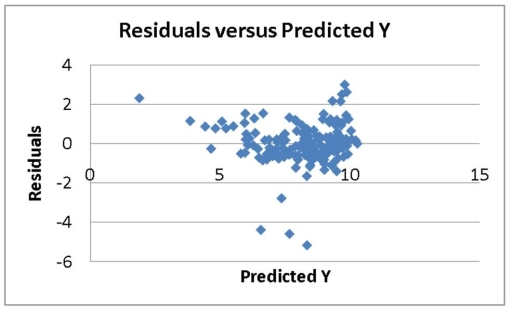
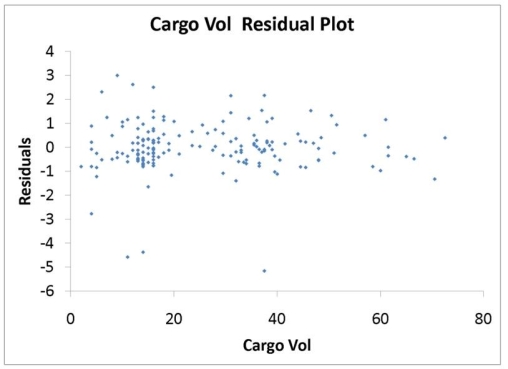
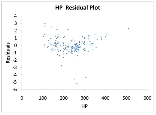
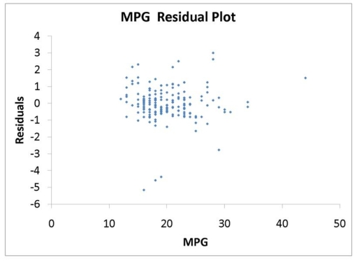
TABLE 14-16 What are the factors that determine the acceleration time (in sec.) from 0 to 60 miles per hour of a car? Data on the following variables for 171 different vehicle models were collected: Accel Time: Acceleration time in sec. Cargo Vol: Cargo volume in cu. ft. HP: Horsepower MPG: Miles per gallon SUV: 1 if the vehicle model is an SUV with Coupe as the base when SUV and Sedan are both 0 Sedan: 1 if the vehicle model is a sedan with Coupe as the base when SUV and Sedan are both 0 The regression results using acceleration time as the dependent variable and the remaining variables as the independent variables are presented below. Regression Statistics Multiple R 0.8013 R Square 0.6421 Adjusted R Square 0.6313 Standard Error 1.0507 Observations 171 $\text { ANOVA }$ df SS MS F Significance F Regression 5 326.8700 65.3740 59.2168 0.0000 Residual 165 182.1564 1.1040 Total 170 509.0263 Coefficients Standard Error t Stat P-value Lower 95\% Upper 95\% Intercept 12.8627 1.0927 11.7713 0.0000 10.7052 15.0202 Cargo Vol 0.0259 0.0102 2.5518 0.0116 0.0059 0.0460 HP -0.0200 0.0018 -11.3307 0.0000 -0.0235 -0.0165 MPG -0.0620 0.0303 -2.0464 0.0423 -0.1218 -0.0022 SUV 0.7679 0.4314 1.7802 0.0769 -0.0838 1.6196 Sedan 0.6427 0.2790 2.3034 0.0225 0.0918 1.1935 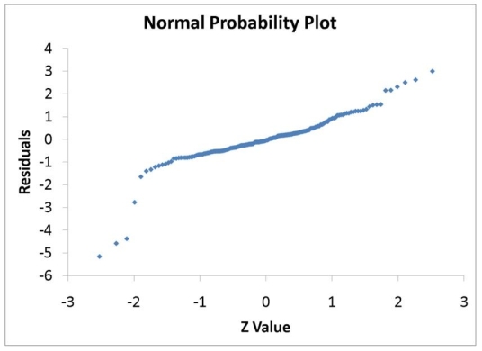The various residual plots are as shown below. The coefficients of partial determination $\left( R ^ { 2 }_{Y j} \right.$ . (All variables except $\left. j \right)$ of each of the 5 predictors are, respectively, $0.0380,0.4376,0.0248,0.0188$ , and $0.0312$ . The coefficient of multiple determination for the regression model using each of the 5 variables $X _ { j }$ as the dependent variable and all other $X$ variables as independent variables $\left( R _ { j } ^ { 2 } \right)$ are, respectively, $0.7461,0.5676,0.6764,0.8582,0.6632$ . -Referring to 14-16, what is the p-value of the test statistic to determine whether HP makes a significant contribution to the regression model in the presence of the other independent variables at a 5% level of significance?

TABLE 14-15 The superintendent of a school district wanted to predict the percentage of students passing a sixth-grade proficiency test. She obtained the data on percentage of students passing the proficiency test (% Passing), daily mean of the percentage of students attending class (% Attendance), mean teacher salary in dollars (Salaries), and instructional spending per pupil in dollars (Spending) of 47 schools in the state. Following is the multiple regression output with Y = % Passing as the dependent variable, X₁ = % Attendance, X₂= Salaries and X₃= Spending: Regression Statistics Multiple R 0.7930 R Square 0.6288 Adjusted R 0.6029 Square Standard 10.4570 Error Observations 47 $\text { ANOVA }$ df SS MS Significance F Regression 3 7965.08 2655.03 24.2802 0.0000 Residual 43 4702.02 109.35 Total 46 12667.11 Coefficients Standard Error t Stat P-value Lower 95\% Upper 95\% Intercept -753.4225 101.1149 -7.4511 0.0000 -957.3401 -549.5050 \% Attendance 8.5014 1.0771 7.8929 0.0000 6.3292 10.6735 Salary 0.000000685 0.0006 0.0011 0.9991 -0.0013 0.0013 Spending 0.0060 0.0046 1.2879 0.2047 -0.0034 0.0153 -Referring to Table 14-15, the alternative hypothesis H?: At least one of ?? ? 0 for j = 0,1,2,3 implies that percentage of students passing the proficiency test is related to all of the explanatory variables.

TABLE 14-17 Given below are results from the regression analysis where the dependent variable is the number of weeks a worker is unemployed due to a layoff (Unemploy) and the independent variables are the age of the worker (Age), the number of years of education received (Edu), the number of years at the previous job (Job Yr), a dummy variable for marital status (Married: 1 = married, 0 = otherwise), a dummy variable for head of household (Head: 1 = yes, 0 = no) and a dummy variable for management position (Manager: 1 = yes, 0 = no). We shall call this Model 1. The coefficients of partial determination ( 2 Yj. (Allvariables except $j$ ) ) of each of the 6 predictors are, respectively, 0.2807, 0.0386, 0.0317, 0.0141, 0.0958, and 0.1201. Regression Statistics Multiple R 0.7035 R Square 0.4949 Adjusted R 0.4030 Square Standard 18.4861 Error 40 Observations $\text { ANOVA }$ df SS MS F significance F Regression 6 11048.6415 1841.4402 5.3885 0.00057 Residual 33 11277.2586 341.7351 Total 39 22325.9 Coefficients Standard Error t Stat P-value Lower 95\% Upper 95\% Intercept 32.6595 23.18302 1.4088 0.1683 -14.5067 79.8257 Age 1.2915 0.3599 3.5883 0.0011 0.5592 2.0238 Edu -1.3537 1.1766 -1.1504 0.2582 -3.7476 1.0402 Job Yr 0.6171 0.5940 1.0389 0.3064 -0.5914 1.8257 Married -5.2189 7.6068 -0.6861 0.4974 -20.6950 10.2571 Head -14.2978 7.6479 -1.8695 0.0704 -29.8575 1.2618 Manager -24.8203 11.6932 -2.1226 0.0414 -48.6102 -1.0303 Model 2 is the regression analysis where the dependent variable is Unemploy and the independent variables are Age and Manager. The results of the regression analysis are given below: Regression Statistics Multiple R 0.6391 R Square 0.4085 Adjusted R 0.3765 Square Standard Error 18.8929 Observations 40 $\text { ANOVA }$ df SS MS F Significance F Regression 2 9119.0897 4559.5448 12.7740 0.0000 Residual 37 13206.8103 356.9408 Total 39 22325.9 Coefficients Standard Error t Stat P -value Intercept -0.2143 11.5796 -0.0185 0.9853 Age 1.4448 0.3160 4.5717 0.0000 Manager -22.5761 11.3488 -1.9893 0.0541 -Referring to Table 14-17 Model 1, the null hypothesis should be rejected at a 10% level of significance when testing whether being married or not makes a difference in the mean number of weeks a worker is unemployed due to a layoff while holding constant the effect of all the other independent variables.

TABLE 14-19 The marketing manager for a nationally franchised lawn service company would like to study the characteristics that differentiate home owners who do and do not have a lawn service. A random sample of 30 home owners located in a suburban area near a large city was selected; 15 did not have a lawn service (code 0) and 15 had a lawn service (code 1). Additional information available concerning these 30 home owners includes family income (Income, in thousands of dollars), lawn size (Lawn Size, in thousands of square feet), attitude toward outdoor recreational activities (Atitude 0 = unfavorable, 1 = favorable), number of teenagers in the household (Teenager), and age of the head of the household (Age). The Minitab output is given below: Logistic Regression Table Odds 95\% CI Predictor Coef SE Coef Z P Ratio Lower Upper Constant -70.49 47.22 -1.49 0.135 Income 0.2868 0.1523 1.88 0.060 1.33 0.99 1.80 LawnSiz 1.0647 0.7472 1.42 0.154 2.90 0.67 12.54 Attitude -12.744 9.455 -1.35 0.178 0.00 0.00 326.06 Teenager -0.200 1.061 -0.19 0.850 0.82 0.10 6.56 Age 1.0792 0.8783 1.23 0.219 2.94 0.53 16.45 Log-Likelihood $= - 4.890$ Test that all slopes are zero: $\mathrm { G } = 31.808 , \mathrm { DF } = 5 , p$ -value $= 0.000$ Goodness-of-Fit Tests Method Chi-Square DF Pearson 9.313 24 0.997 Deviance 9.780 24 0.995 Hosmer-Lemeshow 0.571 8 1.000 -Referring to Table 14-19, what is the p-value of the test statistic when testing whether the model is a good-fitting model?

TABLE 14-3 An economist is interested to see how consumption for an economy (in $ billions) is influenced by gross domestic product ($ billions) and aggregate price (consumer price index). The Microsoft Excel output of this regression is partially reproduced below. SUMMARY OUTPUT Regression Statistics Multiple R 0.991 R Square 0.982 Adjusted R Square 0.976 Standard Error 0.299 Observations 10 ANOVA df SS MS F Signif F Regression 2 33.4163 16.7082 186.325 0.0001 Residual 7 0.6277 0.0897 Total 9 34.0440 Coeff StdError t Stat p -value Intercept -0.0861 0.5674 -0.152 0.8837 GDP 0.7654 0.0574 13.340 0.0001 Price -0.0006 0.0028 -0.219 0.8330 -Referring to Table 14-3, to test whether aggregate price index has a positive impact on consumption, the p-value is

TABLE 14-17 Given below are results from the regression analysis where the dependent variable is the number of weeks a worker is unemployed due to a layoff (Unemploy) and the independent variables are the age of the worker (Age), the number of years of education received (Edu), the number of years at the previous job (Job Yr), a dummy variable for marital status (Married: 1 = married, 0 = otherwise), a dummy variable for head of household (Head: 1 = yes, 0 = no) and a dummy variable for management position (Manager: 1 = yes, 0 = no). We shall call this Model 1. The coefficients of partial determination ( 2 Yj. (Allvariables except $j$ ) ) of each of the 6 predictors are, respectively, 0.2807, 0.0386, 0.0317, 0.0141, 0.0958, and 0.1201. Regression Statistics Multiple R 0.7035 R Square 0.4949 Adjusted R 0.4030 Square Standard 18.4861 Error 40 Observations $\text { ANOVA }$ df SS MS F significance F Regression 6 11048.6415 1841.4402 5.3885 0.00057 Residual 33 11277.2586 341.7351 Total 39 22325.9 Coefficients Standard Error t Stat P-value Lower 95\% Upper 95\% Intercept 32.6595 23.18302 1.4088 0.1683 -14.5067 79.8257 Age 1.2915 0.3599 3.5883 0.0011 0.5592 2.0238 Edu -1.3537 1.1766 -1.1504 0.2582 -3.7476 1.0402 Job Yr 0.6171 0.5940 1.0389 0.3064 -0.5914 1.8257 Married -5.2189 7.6068 -0.6861 0.4974 -20.6950 10.2571 Head -14.2978 7.6479 -1.8695 0.0704 -29.8575 1.2618 Manager -24.8203 11.6932 -2.1226 0.0414 -48.6102 -1.0303 Model 2 is the regression analysis where the dependent variable is Unemploy and the independent variables are Age and Manager. The results of the regression analysis are given below: Regression Statistics Multiple R 0.6391 R Square 0.4085 Adjusted R 0.3765 Square Standard Error 18.8929 Observations 40 $\text { ANOVA }$ df SS MS F Significance F Regression 2 9119.0897 4559.5448 12.7740 0.0000 Residual 37 13206.8103 356.9408 Total 39 22325.9 Coefficients Standard Error t Stat P -value Intercept -0.2143 11.5796 -0.0185 0.9853 Age 1.4448 0.3160 4.5717 0.0000 Manager -22.5761 11.3488 -1.9893 0.0541 -Referring to Table 14-17 Model 1, we can conclude that, holding constant the effect of the other independent variables, there is a difference in the mean number of weeks a worker is unemployed due to a layoff between a worker who is married and one who is not at a 5% level of significance if we use only the information of the 95% confidence interval estimate for ??.