Exam 16: Time-Series Forecasting
Exam 1: Introduction145 Questions
Exam 2: Organizing and Visualizing Data210 Questions
Exam 3: Numerical Descriptive Measures153 Questions
Exam 4: Basic Probability171 Questions
Exam 5: Discrete Probability Distributions218 Questions
Exam 6: The Normal Distribution and Other Continuous Distributions191 Questions
Exam 7: Sampling and Sampling Distributions197 Questions
Exam 8: Confidence Interval Estimation196 Questions
Exam 9: Fundamentals of Hypothesis Testing: One-Sample Tests165 Questions
Exam 10: Two-Sample Tests210 Questions
Exam 11: Analysis of Variance213 Questions
Exam 12: Chi-Square Tests and Nonparametric Tests201 Questions
Exam 13: Simple Linear Regression213 Questions
Exam 14: Introduction to Multiple Regression355 Questions
Exam 15: Multiple Regression Model Building96 Questions
Exam 16: Time-Series Forecasting168 Questions
Exam 17: Statistical Applications in Quality Management133 Questions
Exam 18: A Roadmap for Analyzing Data54 Questions
Select questions type
Based on the following scatter plot, which of the time-series components is not present in this quarterly time series? 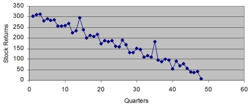
Free
(Multiple Choice)
4.9/5  (23)
(23)
Correct Answer: Verified
C
TABLE 16-10 Business closures in Laramie, Wyoming from 2005 to 2010 were: 2005 10 2006 11 2007 13 2008 19 2009 24 2010 35
Microsoft Excel was used to fit both first-order and second-order autoregressive models, resulting in the following partial outputs:
SUMMARY OUTPUT - 2nd Order Model
Coefficient Intercept -5.77 X Variable 1 0.80 X Variable 2 1.14
SUMMARY OUTPUT - 1 st Order Model
Coefficients Intercept -4.16 X Variable 1 1.59
-Referring to Table 16-10, the value of the MAD for the first-order autoregressive model is ________.
Free
(Short Answer)
4.8/5 (39)
Correct Answer:Verified
1.322
Which of the following terms describes the up and down movements of a time series that vary both in length and intensity?
Free
(Multiple Choice)
4.8/5 (35)
Correct Answer:Verified
B
TABLE 16-12
A local store developed a multiplicative time-series model to forecast its revenues in future quarters, using quarterly data on its revenues during the 4-year period from 2005 to 2009. The following is the resulting regression equation:
log₁₀ = 6.102 + 0.012 X - 0.129 Q₁ - 0.054 Q₂ + 0.098 Q₃
where is the estimated number of contracts in a quarter.
X is the coded quarterly value with X = 0 in the first quarter of 2005.
Q₁ is a dummy variable equal to 1 in the first quarter of a year and 0 otherwise.
Q₂ is a dummy variable equal to 1 in the second quarter of a year and 0 otherwise.
Q₃ is a dummy variable equal to 1 in the third quarter of a year and 0 otherwise.
-Referring to Table 16-12, using the regression equation, what is the forecast for the revenues in the third quarter of 2010?
(Short Answer)
4.9/5 (34)
Which of the following methods should not be used for short-term forecasts into the future?
(Multiple Choice)
4.9/5 (38)
A first-order autoregressive model for stock sales is:
Salesᵢ = 800 + 1.2(Sales)ᵢ₋₁.
If sales in 2010 is 6,000, the forecast of sales for 2011 is ________.
(Short Answer)
4.9/5 (33)
TABLE 16-4
The number of cases of merlot wine sold by a Paso Robles winery in an 8-year period follows.
Year Cases of Wine 2003 270 2004 356 2005 398 2006 456 2007 358 2008 500 2009 410 2010 376
-Referring to Table 16-4, a centered 5-year moving average is to be constructed for the wine sales. The number of moving averages that will be calculated is ________.
(Short Answer)
4.9/5 (27)
TABLE 16-14
A contractor developed a multiplicative time-series model to forecast the number of contracts in future quarters, using quarterly data on number of contracts during the 3-year period from 2008 to 2010. The following is the resulting regression equation:
ln Ŷ = 3.37 + 0.117 X - 0.083 Q₁ + 1.28 Q₂ + 0.617 Q₃
where Ŷ is the estimated number of contracts in a quarter
X is the coded quarterly value with X = 0 in the first quarter of 2008.
Q₁ is a dummy variable equal to 1 in the first quarter of a year and 0 otherwise.
Q₂ is a dummy variable equal to 1 in the second quarter of a year and 0 otherwise.
Q₃ is a dummy variable equal to 1 in the third quarter of a year and 0 otherwise.
-Referring to Table 16-14, using the regression equation, which of the following values is the best forecast for the number of contracts in the second quarter of 2012?
(Multiple Choice)
4.9/5 (33)
Each forecast using the method of exponential smoothing depends on all the previous observations in the time series.
(True/False)
4.9/5 (40)
If a time series does not exhibit a long-term trend, the method of exponential smoothing may be used to obtain short-term predictions about the future.
(True/False)
4.7/5 (27)
A model that can be used to make predictions about long-term future values of a time series is
(Multiple Choice)
4.7/5 (39)
TABLE 16-13
Given below is the monthly time-series data for U.S. retail sales of building materials over a specific year.
Month Retail Sales 1 6,594 2 6,610 3 8,174 4 9,513 5 10,595 6 10,415 7 9,949 8 9,810 9 9,637 10 9,732 11 9,214 12 9,201
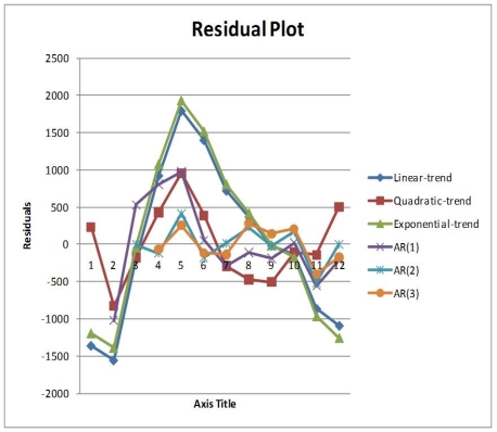
The results of the linear trend, quadratic trend, exponential trend, first-order autoregressive, second-order autoregressive and third-order autoregressive model are presented below in which the coded month for the first month is 0:
Coefficients Standard Error t Stat P-value Intercept 7950.7564 617.6342 12.8729 0.0000 Coded Month 212.6503 95.1145 2.2357 0.0494
Quadratic trend model:
Coefficients Standard Error t Stat P-value Intercept 6358.2473 417.2692 15.2378 0.0000 Coded Month 1168.1558 176.3526 6.6240 0.0001 Coded Month 2 -86.8641 15.4474 -5.6232 0.0003
Exponential trend model:
Coefficients Standard Error t Stat P-value Intercept 3.8912 0.0315 123.3674 0.0000 Coded Month 0.0116 0.0049 2.3957 0.0376
Coefficients Standard Error t Stat P-value Intercept 3132.0951 1287.2899 2.4331 0.0378 YLag1 0.6823 0.1398 4.8812 0.0009
Second-order autoregressive::
Coefficients Standard Error t Stat P -value Intercept 4968.5789 766.9416 6.4784 0.0003 YLag1 0.9333 0.1547 6.0316 0.0005 YLag2 -0.4487 0.1238 -3.6235 0.0085
Third-order autoregressive::
Coefficients Standard Error t Stat P-value Intercept 6782.7567 2105.7115 3.2211 0.0234 YLag1 0.5481 0.3918 1.3990 0.2207 YLag2 0.0198 0.4034 0.0490 0.9628 YLag3 -0.2749 0.2234 -1.2308 0.2731
Below is the residual plot of the various models:
 -Referring to Table 16-13, what is the exponentially smoothed value for the 12ᵗʰ month using a smoothing coefficient of W = 0.25 if the exponentially smooth value for the 10ᵗʰ and 11ᵗʰ month are 9,477.7776 and 9,411.8332, respectively?
(Short Answer)
4.7/5 (31)
TABLE 16-6
The president of a chain of department stores believes that her stores' total sales have been showing a linear trend since 1990. She uses Microsoft Excel to obtain the partial output below. The dependent variable is sales (in millions of dollars), while the independent variable is coded years, where 1990 is coded as 0, 1991 is coded as 1, etc.
SUMMARY OUTPUT
Regression Statistics
Multiple R 0.604 R Square 0.365 Adjusted R Square 0.316 Standard Error 4.800 Observations 17
Coefficients Intercept 31.2 Coded Year 0.78
-Referring to Table 16-6, the estimate of the amount by which sales (in millions of dollars)is increasing each year is ________.
(Short Answer)
4.8/5 (37)
TABLE 16-13
Given below is the monthly time-series data for U.S. retail sales of building materials over a specific year.
Month Retail Sales 1 6,594 2 6,610 3 8,174 4 9,513 5 10,595 6 10,415 7 9,949 8 9,810 9 9,637 10 9,732 11 9,214 12 9,201
The results of the linear trend, quadratic trend, exponential trend, first-order autoregressive, second-order autoregressive and third-order autoregressive model are presented below in which the coded month for the first month is 0:
Coefficients Standard Error t Stat P-value Intercept 7950.7564 617.6342 12.8729 0.0000 Coded Month 212.6503 95.1145 2.2357 0.0494
Quadratic trend model:
Coefficients Standard Error t Stat P-value Intercept 6358.2473 417.2692 15.2378 0.0000 Coded Month 1168.1558 176.3526 6.6240 0.0001 Coded Month 2 -86.8641 15.4474 -5.6232 0.0003
Exponential trend model:
Coefficients Standard Error t Stat P-value Intercept 3.8912 0.0315 123.3674 0.0000 Coded Month 0.0116 0.0049 2.3957 0.0376
Coefficients Standard Error t Stat P-value Intercept 3132.0951 1287.2899 2.4331 0.0378 YLag1 0.6823 0.1398 4.8812 0.0009
Second-order autoregressive::
Coefficients Standard Error t Stat P -value Intercept 4968.5789 766.9416 6.4784 0.0003 YLag1 0.9333 0.1547 6.0316 0.0005 YLag2 -0.4487 0.1238 -3.6235 0.0085
Third-order autoregressive::
Coefficients Standard Error t Stat P-value Intercept 6782.7567 2105.7115 3.2211 0.0234 YLag1 0.5481 0.3918 1.3990 0.2207 YLag2 0.0198 0.4034 0.0490 0.9628 YLag3 -0.2749 0.2234 -1.2308 0.2731
Below is the residual plot of the various models:
-Referring to Table 16-13, the best autoregressive model using the 5% level of significance is
(Multiple Choice)
4.9/5 (41)
TABLE 16-12
A local store developed a multiplicative time-series model to forecast its revenues in future quarters, using quarterly data on its revenues during the 4-year period from 2005 to 2009. The following is the resulting regression equation:
log₁₀ = 6.102 + 0.012 X - 0.129 Q₁ - 0.054 Q₂ + 0.098 Q₃
where is the estimated number of contracts in a quarter.
X is the coded quarterly value with X = 0 in the first quarter of 2005.
Q₁ is a dummy variable equal to 1 in the first quarter of a year and 0 otherwise.
Q₂ is a dummy variable equal to 1 in the second quarter of a year and 0 otherwise.
Q₃ is a dummy variable equal to 1 in the third quarter of a year and 0 otherwise.
-Referring to Table 16-12, the estimated quarterly compound growth rate in revenues is around
(Multiple Choice)
4.9/5 (38)
TABLE 16-13
Given below is the monthly time-series data for U.S. retail sales of building materials over a specific year.
Month Retail Sales 1 6,594 2 6,610 3 8,174 4 9,513 5 10,595 6 10,415 7 9,949 8 9,810 9 9,637 10 9,732 11 9,214 12 9,201
The results of the linear trend, quadratic trend, exponential trend, first-order autoregressive, second-order autoregressive and third-order autoregressive model are presented below in which the coded month for the first month is 0:
Coefficients Standard Error t Stat P-value Intercept 7950.7564 617.6342 12.8729 0.0000 Coded Month 212.6503 95.1145 2.2357 0.0494
Quadratic trend model:
Coefficients Standard Error t Stat P-value Intercept 6358.2473 417.2692 15.2378 0.0000 Coded Month 1168.1558 176.3526 6.6240 0.0001 Coded Month 2 -86.8641 15.4474 -5.6232 0.0003
Exponential trend model:
Coefficients Standard Error t Stat P-value Intercept 3.8912 0.0315 123.3674 0.0000 Coded Month 0.0116 0.0049 2.3957 0.0376
Coefficients Standard Error t Stat P-value Intercept 3132.0951 1287.2899 2.4331 0.0378 YLag1 0.6823 0.1398 4.8812 0.0009
Second-order autoregressive::
Coefficients Standard Error t Stat P -value Intercept 4968.5789 766.9416 6.4784 0.0003 YLag1 0.9333 0.1547 6.0316 0.0005 YLag2 -0.4487 0.1238 -3.6235 0.0085
Third-order autoregressive::
Coefficients Standard Error t Stat P-value Intercept 6782.7567 2105.7115 3.2211 0.0234 YLag1 0.5481 0.3918 1.3990 0.2207 YLag2 0.0198 0.4034 0.0490 0.9628 YLag3 -0.2749 0.2234 -1.2308 0.2731
Below is the residual plot of the various models:
-Referring to Table 16-13, if a five-month moving average is used to smooth this series, what would be the last calculated value?
(Short Answer)
4.7/5 (34)
TABLE 16-13
Given below is the monthly time-series data for U.S. retail sales of building materials over a specific year.
Month Retail Sales 1 6,594 2 6,610 3 8,174 4 9,513 5 10,595 6 10,415 7 9,949 8 9,810 9 9,637 10 9,732 11 9,214 12 9,201
The results of the linear trend, quadratic trend, exponential trend, first-order autoregressive, second-order autoregressive and third-order autoregressive model are presented below in which the coded month for the first month is 0:
Coefficients Standard Error t Stat P-value Intercept 7950.7564 617.6342 12.8729 0.0000 Coded Month 212.6503 95.1145 2.2357 0.0494
Quadratic trend model:
Coefficients Standard Error t Stat P-value Intercept 6358.2473 417.2692 15.2378 0.0000 Coded Month 1168.1558 176.3526 6.6240 0.0001 Coded Month 2 -86.8641 15.4474 -5.6232 0.0003
Exponential trend model:
Coefficients Standard Error t Stat P-value Intercept 3.8912 0.0315 123.3674 0.0000 Coded Month 0.0116 0.0049 2.3957 0.0376
Coefficients Standard Error t Stat P-value Intercept 3132.0951 1287.2899 2.4331 0.0378 YLag1 0.6823 0.1398 4.8812 0.0009
Second-order autoregressive::
Coefficients Standard Error t Stat P -value Intercept 4968.5789 766.9416 6.4784 0.0003 YLag1 0.9333 0.1547 6.0316 0.0005 YLag2 -0.4487 0.1238 -3.6235 0.0085
Third-order autoregressive::
Coefficients Standard Error t Stat P-value Intercept 6782.7567 2105.7115 3.2211 0.0234 YLag1 0.5481 0.3918 1.3990 0.2207 YLag2 0.0198 0.4034 0.0490 0.9628 YLag3 -0.2749 0.2234 -1.2308 0.2731
Below is the residual plot of the various models:
-Referring to Table 16-13, what is the exponentially smoothed value for the first month using a smoothing coefficient of W = 0.25?
(Short Answer)
4.8/5 (36)
TABLE 16-3
The following table contains the number of complaints received in a department store for the first 6 months of last year.
Month Complaints January 36 February 45 March 81 April 90 May 108 June 144
-Referring to Table 16-3, if this series is smoothed using exponential smoothing with a smoothing constant of 1/3, what would be the second value?
(Multiple Choice)
4.7/5 (34)
TABLE 16-12
A local store developed a multiplicative time-series model to forecast its revenues in future quarters, using quarterly data on its revenues during the 4-year period from 2005 to 2009. The following is the resulting regression equation:
log₁₀ = 6.102 + 0.012 X - 0.129 Q₁ - 0.054 Q₂ + 0.098 Q₃
where is the estimated number of contracts in a quarter.
X is the coded quarterly value with X = 0 in the first quarter of 2005.
Q₁ is a dummy variable equal to 1 in the first quarter of a year and 0 otherwise.
Q₂ is a dummy variable equal to 1 in the second quarter of a year and 0 otherwise.
Q₃ is a dummy variable equal to 1 in the third quarter of a year and 0 otherwise.
-Referring to Table 16-12, using the regression equation, what is the forecast for the revenues in the first quarter of 2012?
(Short Answer)
4.8/5 (36)
Which of the following terms describes the overall long-term tendency of a time series?
(Multiple Choice)
4.8/5 (32)
Filters
- Essay(0)
- Multiple Choice(0)
- Short Answer(0)
- True False(0)
- Matching(0)