Exam 13: Asking and Answering Questions About the Difference Between Two Means

The $P$ -value for a hypothesis test is always found by calculating areas under the $z$ curve.

When wildlife biologists study small animals, the animals are trapped and then anesthetized to prevent discomfort to the animal. A study of the effect of the anesthetic, Isoflurane, on eastern gray squirrels (Sciurus carolinensis) resulted in the pulse data presented below. The biologists were interested in comparing the effects of Isoflurane in two different seasons, winter and summer. Pulse (heartbeats/min) Group Sample size Mean Standard deviation Summer 43 324.6 128.17 Winter 48 373.2 50.49 An initial analysis of the data revealed that it was reasonable to assume the distribution of pulses for each season is approximately normal. It was also judged to be reasonable to regard these samples as representative of the eastern gray squirrel population. a) Test the hypothesis of no difference in eastern gray squirrel mean pulse for winter and summer. b) Do the data indicate that the mean pulse differs for the two seasons? Provide an appropriate statistical justification using your response in part (a).

"Tail-chasing" by dogs is an anxiety disorder characterized by circling behavior with the dog's attention directed toward its tail. There may be many reasons for tail- chasing behaviors. To investigate the potential for biochemical causes, a study was performed at a small animal clinic at a university. Blood samples were taken from a random sample of 15 dogs brought to the clinic by owners worried about the tail- chasing behaviors of their dogs. A control group consisting of a random sample of 15 dogs brought to the clinic for other reasons contributed blood samples with the owner's permission. The mean triglyceride level for the tail-chasing group was 68 mg/dl, and the standard deviation was 19.36 mg/dl. The corresponding statistics for the control group were 61 mg/dl and 11.62 mg/dl. Both sample distributions were approximately symmetric. a) Is there convincing evidence of a difference in mean triglyceride level in these two populations? Provide statistical justification for your response. b) Irrespective of your response in part (a), consider the design of this study. Would a statistically significant difference in mean triglyceride levels be sufficient to make a case that triglyceride level is a cause of tail-chasing behavior in dogs? Why or why not?

The estimated standard deviation of $\bar { x } _ { 1 } - \bar { x } _ { 2 }$ used in hypothesis tests about $\mu _ { 1 } - \mu _ { 2 }$ is the same as the estimated standard deviation used in calculating confidence intervals for $\mu _ { 1 } - \mu _ { 2 }$ .

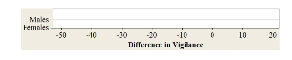
When stalking gazelles, cheetah frequently have a choice between two gazelles close to each other while grazing. A biologist thought the choice of prey might be affected by the "vigilance" behavior of the gazelles. She defined vigilance as the percentage of the time that a gazelle had its head in the air searching for potential predators. She filmed cheetah stalks and analyzed 16 incidents where two same-sex gazelles were within 5 meters of each other; thus, either could have been chosen as the cheetah's prey. The table below presents the vigilance levels for each of the gazelles and the difference (gazelle chased - gazelle ignored) for each pair. Vigilance of Vigilance of Difference Pair the the In sex \# Gazelle Gazelle Vigilance Chased Ignored 8.0 10.0 -2.0 Male 31.4 78.7 -47.3 Male 40.0 52.0 -12.0 Male 15.7 23.9 -8.2 Male 40.0 81.0 -41.0 Male 35.3 49.7 -14.4 Male 31.7 62.0 -30.3 Male 68.5 72.6 -4.1 Male 45.0 96.3 -51.3 Male 39.1 90.1 -51.0 Male 65.2 88.3 -23.1 Male 72.5 89.9 -17.4 Male 17.5 65.0 -47.5 Female 63.0 84.2 -21.2 Female 70.2 50.0 20.2 Female 38.8 20.5 18.3 Female a) Using the scales below, construct comparative dotplots to show that it is reasonable to use the $t$ -procedure to construct confidence intervals for the difference in population means for males and females. b) Calculate and interpret the 95% confidence interval in the context of the problem. c) The investigator noticed that many more male pairs than female pairs were actually stalked by cheetah. Two theories have been proposed for this difference. The first theory is that the gazelle females are generally more vigilant than males. The second theory is that females generally graze near the centers of the herds, protecting the young, and are less accessible to predators. i) Is it possible to use investigator's data be used to support or refute the theory that females are more vigilant than males? Is so, how? If not, why not? ii) Is it possible to use investigator's data be used to support or refute the theory that females generally graze near the centers of the herds? Is so, how? If not, why not?

In a study of captive nectar-feeding bats (Leptonycteris sanborni), data were gathered on nectar intake over a five-minute flight period. The bats were randomly selected for the study. Investigators are interested in the differences in weight gain for males and females. The bats were weighed before and after feeding, and the relative weight gain was calculated for each animal using the formula: $R W G=\frac{\text { PostFeeding - Original }}{\text { Original }}$ Bat \# Sex Original Weight Post-feeding Weight Relative Weight gain 18.6 19.8 0.065 18.5 20.8 0.124 18.6 20.0 0.075 20.4 21.9 0.074 21.5 23.0 0.070 20.3 22.0 0.084 F 17.0 18.5 0.088 17.0 19.0 0.118 17.5 19.2 0.097 19.7 21.0 0.066 18.2 20.2 0.110 20.2 22.3 0.104 19.0 20.5 0.079 17.3 18.5 0.069 17.8 19.0 0.067 19.5 21.6 0.108 21.0 22.8 0.086 17.0 18.4 0.082 18.3 19.3 0.055 Consider constructing a $95 \%$ confidence interval for the population difference in mean weight gains for male and female bats. a) Using a graphic display of your choice, show that it is appropriate to use the $t$ procedure to construct a confidence interval. b) Calculate and interpret the $95 \%$ confidence interval in the context of the problem. c) Do you feel these results can be generalized to non-captive bats? Why or why not?

For both large and small samples the estimated standard deviation of $\bar { x } _ { 1 } - \bar { x } _ { 2 }$ is calculated the same way.

"Tail-chasing" by dogs is an anxiety disorder characterized by circling behavior with the dog's attention directed toward its tail. There may be many reasons for tail- chasing behaviors. To investigate the potential for biochemical causes, a study was performed at a small animal clinic at a university. Blood samples were taken from random sample of 15 dogs brought to the clinic by owners worried about the tail- chasing behaviors of their dogs. A control group consisting of a random sample of 15 dogs brought to the clinic for other reasons contributed blood samples with the owner's permission. The mean lipoprotein density for the tail-chasing group was 12 mg/dl, and the standard deviation was 2.24 mg/dl. The corresponding statistics for the control group were 13 mg/dl and 1.73 mg/dl. There was no indication of skewness in either sample distribution. a) Is there sufficient evidence to conclude that there is a difference in mean lipoprotein density in these two samples? Provide statistical justification for your response. b) Irrespective of your response in part (a), consider the design of this study. Would a statistically significant difference in mean lipoprotein density be sufficient to make a case that lipoprotein density is the cause of tail-chasing behavior in dogs? Why or why not?

A number of butterfly species mate for hours, and if a mating couple is disturbed, one of the butterflies is responsible for flying, carrying its partner with it. Not only are mating pairs more noticeable to predators, but the added weight may hamper the flight during escape. Random samples of Green-veined White (Pieris napi) butterflies were the subjects of a Swedish study to investigate the escape flights of single butterflies and of mating pairs when exposed to a predator. Data on the initial takeoff escape velocities are presented below. The investigators considered performing a hypothesis test to determine if there was evidence that the mean take off escape velocity was different for singles and pairs. Using a graphical procedure of your choice, determine if the t-test is appropriate. Escape velocity (m/sec) Single 0.76,0.89,0.94,1.01,1.09,1.11,1.12,1.17,1.19,1.20,1.29 1.34,1.42,1.54 Paired 0.58,0.58,0.76,0.86,0.95,0.97,1.03,1.05,1.14,1.35,1.38 1.61,1.62,1.77,2.29,2.29

Inferences about the difference between two means fall into two categories: the samples are independent, or the samples are paired. a) What considerations would lead you to use the techniques for independent samples rather than those for paired samples? You may use examples to illustrate your ideas, but examples alone are not sufficient. b) How do the analyses of independent samples and paired samples differ? In your response, consider the hypotheses, methods, assumptions, and calculations.

In many animal species the males and females differ slightly in structure, coloring, and/or size. The hominid species Australopithecus is thought to have lived about 3.2 million years ago. ("Lucy," the famous near-complete skeleton discovered in 1974, is an Australopithecus.) Forensic anthropologists use partial skeletal remains to estimate the mass of an individual. The data below are estimates of masses from partial skeletal remains of this species found in sub-Saharan Africa. Appropriate graphical displays of the data indicate that it is reasonable to assume that the population distributions of mass are approximately normal for both males and females. You may also assume that these samples are representative of the respective populations. Estimates of mass (kg) Males 51.0 45.4 45.6 50.1 41.3 42.6 40.2 48.2 38.4 45.4 40.7 37.9 41.3 31.5 Females 27.1 33.5 28.0 30.3 32.7 32.5 34.2 30.5 27.5 23.3 35.7 Do these data provide convincing evidence that the mean estimated masses differ for Australopithecus males and females? Provide appropriate statistical justification for your conclusion.

When wildlife biologists study small animals, the animals are trapped and then anesthetized to prevent discomfort to the animal. A study of the effect of the anesthetic, Isoflurane, on Allegheny woodrats (Neotoma magister) resulted in the heartbeat data presented below. The biologists were interested in comparing the effects of Isoflurane in two different seasons, winter and summer. Heartbeat Rate (heartbeats/min) Group Sample size Mean Standard deviation Summer 24 347.5 80.83 Winter 13 360.0 133.04 An initial analysis of the data revealed that it was reasonable to assume the distributions of heartbeats for both seasons are approximately normal. It was also judged to be reasonable to regard these samples as representative of the Allegheny woodrat population. a) Test the hypothesis of no difference between woodrat mean heartbeat rates for winter and summer. b) Do the data indicate that the mean heartbeat rates differ? Provide an appropriate statistical justification using your response in part (a).

Researchers usually test the hypothesis $H _ { o } : \bar { x } _ { 1 } - \bar { x } _ { 2 } = 0$ with an alternative hypothesis of $H _ { a } : \bar { x } _ { 1 } - \bar { x } _ { 2 } \neq 0$ rather than using a one-sided alternative.

$\bar { x } _ { 1 } - \bar { x } _ { 2 } \text { is an unbiased statistic used to estimate } \mu _ { 1 } - \mu _ { 2 } \text {. }$ $\text { For two independent samples, } \sigma _ { \bar { x } _ { 1 } - \bar { x } _ { 2 } } = \sqrt { \frac { \sigma _ { 1 } ^ { 2 } } { n _ { 1 } } - \frac { \sigma _ { 2 } ^ { 2 } } { n _ { 2 } } } \text {. }$

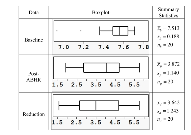
After an outbreak of a drug-resistant strain of bacteria (Enterococci faecium), hospital officials became concerned that their alcohol-based handrub (ABHR) hand hygiene program was not sufficient to prevent spreading this bacteria. The officials solicited 20 volunteers to assess the effectiveness of ABHR. The volunteers' hands were contaminated with $E$ . faecium. After gathering baseline data on the amount of bacteria present they performed the recommended hand hygiene according to the World Health Organization protocol. The amount of bacteria present was then assessed again. Summary measures and boxplots of the baseline sample, the postABHR sample, and the reduction in the amount of bacteria ( $\log _ { 10 } ($ bacteria $\left. / \mathrm { mL } ) \right)$ are presented below. Do these data provide sufficient evidence that the ABHR is effective against the E. faecium?

A number of butterfly species mate for hours, and if a mating couple is disturbed, one of the butterflies is responsible for flying, carrying its partner with it. Not only are mating pairs more noticeable to predators, the added weight may hamper the flight during escape. Random samples of Green-veined White (Pieris napi) butterflies were the subjects of a Swedish study to investigate the escape flights of single butterflies and of mating pairs when exposed to a predator. Data on the initial takeoff angle of escape are presented below. The investigators considered performing a hypothesis test to determine if there was evidence that the mean take off angle was different for singles and pairs. Using a graphical procedure of your choice, determine if the t-test is appropriate. $\text { Take-off angle (degrees) }$ Take-off angle (degrees) Single 0.4, 1.9, 7.0, 21.7 24.4, 28.0, 28.6, 35.4, 39.9, 40.2, 57.0 57.0, 65.0, 68.9 Paired 1.0, 8.5, 8.5, 13.9, 14.8, 15.7, 16.6, 25.3, 29.5, 36.0, 44.7 47.1, 51.6, 55.8, 73.1, 74.3

In an introductory marketing class students were presented with 6 items they could bid on in an auction. They were asked to bid privately and also estimate the "typical" bid for each item by their classmates. The items were randomly selected from a large list of items that students might purchase. An initial analysis of the data established the plausibility that the distribution of differences (estimated - actual) is approximately normal. Actual \& Estimated Median Bids (\$) for Typical Goods Good Actual Estimated Diff Teddy Bear 1.00 4.90 3.9 Music CD 1.25 4.53 3.28 Red velvet 2.70 5.44 2.74 Sachet Soma wooden puzzle 3.00 5.17 2.17 8 smoked Salmon 3.00 6.67 3.67 1 lb Jelly Bellies 4.00 7.30 3.3 a)Construct a $95 \%$ confidence interval for the mean difference between the actual bid and the estimated "typical" bid for the population of items. b) Do the data indicate that the mean differs for the actual and estimated "typical" bids? Provide an appropriate statistical justification using your response in part (a).

Generally speaking, the "pooled" $t$ is preferred if population variances are unequal.

When an alternative hypothesis is $H _ { a } : \mu _ { 1 } - \mu _ { 2 } \neq 0$ the $P$ -value is found by doubling the appropriate area under the $t$ curve.

The number of degrees of freedom associated with the two-sample $t$ test is the same as the number of degrees of freedom associated with the paired $t$ test statistic.