Exam 6: Random Variables and Probability Distributions

At the last home football game of the season, the senior football players walk through a specially constructed welcoming arch, 2 abreast. The arch is 50" wide. It is considered unseemly to bump each other on the way through, so the arch must be wide enough for two players to go through. The distribution of widths of football players with shoulder pads is approximately normal with a mean of 30 inches, and the standard deviation is 5 inches. Let random variable w = width in inches of a randomly selected padded football player. a) The carpenter who will be constructing the arch has only metric measuring tools, and must convert all the information above to metric measures. Let random variable $m =$ width in centimeters of a randomly selected padded football player. What are the mean and standard deviation of $m$ ? (Note: 1 inch $= 2.54$ centimeters) b) Suppose the football players are paired randomly to go through the arch. Define random variable $v = w _ { 1 } + w _ { 2 }$ to be the collective width -- in inches -- of two randomly selected football players. What are the mean and standard deviation of $v$ ? c) The original specifications of the arch specified a 10 inch separation of the players so that they have room to avoid each other. Define the random variable, "amount" of room needed for two football players: $a = 10 + w _ { 1 } + w _ { 2 }$ . How does the mean and standard deviation in part (b) differ from the mean and standard deviation of the random variable, $a$ ? Do not recalculate the mean and standard deviation. d) The school safety committee is concerned about the amount of "wiggle" room in the arch. The wiggle room is the amount of space left over when two players go through the arch. Using your results from (b) and (c) above, define a random variable, $g$ , which the committee could use in their analysis of the amount of wiggle room.

Free

(Essay)

4.8/5

(34)

Question 1

Correct Answer:

Verified

a)
$\begin{array} { l } \mu _ { c m } = ( 2.54 ) ( 30 ) = 76.2 \\\sigma _ { c m } = ( 2.54 ) ( 5 ) = 12.7\end{array}$
b)
$\begin{array} { l } \mu _ { w + w } = \mu _ { w } + \mu _ { w } = 60 \\\sigma _ { w + w } ^ { 2 } = \sigma _ { w } ^ { 2 } + \sigma _ { w } ^ { 2 } = 50 \\\sigma _ { w } = 7.071\end{array}$
c) The mean is increased by 10 ; the standard deviation is unchanged.

One theory of why birds form in flocks is that flocks increase efficiency in scanning for approaching predators. Because birds can barely move their eyes they must turn their heads to look for predators, making them temporarily unable to peck for food. If the birds form flocks, each bird could spend less time scanning; when a single bird detects a predator it alerts the other birds. The Chanting Goshawk is a predator of the Red-billed Weaver bird. From field observation it is estimated that an individual weaver bird has a probability of 0.20 of detecting a goshawk in time to fly to safety. Suppose that a goshawk suddenly comes upon a flock of 4 weaver birds pecking for food on the ground, and attacks. a) What is the probability that none of the weaver birds will detect the goshawk's presence before it is too late, thus allowing the goshawk to have a weaver bird lunch? b) What is the probability that at least one of the weaver birds will detect the goshawk's presence, thus alerting the others and all fly away, leaving the goshawk hungry? c) Suppose this is Wednesday, and all weaver birds form flocks of size 4 on Wednesdays. Using your results from parts (a) and/or (b), find the probability that a goshawk will go hungry until swooping down on the 5th flock of 4 weaver birds seen that day.

Free

(Essay)

4.8/5

(34)

Question 2

Correct Answer:

Verified

a) $( 0.8 ) ^ { 4 } = 0.4096$
b) $1 - ( 0.8 ) ^ { 4 } = 0.5904$
c) $( 0.5904 ) ^ { 4 } ( 0.4096 ) = 0.4977$

Road construction in the town of Hiawatha has presented some problems for the traffic engineers. Small businesses such as Joe's Barber Shop will require an alternate entrance for their customers. This will in turn create a minor congestion of traffic nearby because cars will be backed up and the entrance to the parking lot. The engineers have studied the problem using simulations based on current traffic patterns. The results from 500 trials are shown below: Number of times cars are backed up at the entrance 0 300 1 100 2 75 3 25 Let the random variable k = number of cars backed up at the entrance. a) Fill in the table below with the estimated probability distribution of k, and sketch a probability histogram for x. Probability distribution k (x) 0 1 2 3 Probability histogram $Road construction in the town of Hiawatha has presented some problems for the traffic engineers. Small businesses such as Joe's Barber Shop will require an alternate entrance for their customers. This will in turn create a minor congestion of traffic nearby because cars will be backed up and the entrance to the parking lot. The engineers have studied the problem using simulations based on current traffic patterns. The results from 500 trials are shown below: \begin{array} { | c | c | } \hline \boldsymbol { k } & \begin{array} { l } \text { Number of times } \boldsymbol { k } \\ \text { cars are backed up } \\ \text { at the entrance } \end{array} \\ \hline 0 & 300 \\ 1 & 100 \\ 2 & 75 \\ 3 & 25 \\ \hline \end{array} Let the random variable k = number of cars backed up at the entrance. a) Fill in the table below with the estimated probability distribution of k, and sketch a probability histogram for x. Probability distribution \begin{array}{|l|l|} \hline k & \mathbf{P}(x) \\ \hline 0 & \\ \hline 1 & \\ \hline 2 & \\ \hline 3 & \\ \hline \end{array} Probability histogram b) Using the estimated probabilities in part (a), calculate the following: i) P ( k = 1 ) , the probability that 1 car is backed up at the entrance. ii) P ( x < 2 ) , the probability that fewer than 2 cars are backed up at the entrance iii) P ( x \geq 1 ) , the probability that at least 1 car is backed up at the entrance$ b) Using the estimated probabilities in part (a), calculate the following: i) $P ( k = 1 )$ , the probability that 1 car is backed up at the entrance. ii) $P ( x < 2 )$ , the probability that fewer than 2 cars are backed up at the entrance iii) $P ( x \geq 1 )$ , the probability that at least 1 car is backed up at the entrance

Free

(Essay)

4.8/5

(33)

Question 3

Correct Answer:

Verified

a) Graph should be consistent with these values. $\begin{array} { | c | c | } \hline k & \mathrm { P } ( x ) \\\hline 0 & .60 \\\hline 1 & .20 \\\hline 2 & .15 \\\hline 3 & .05 \\\hline\end{array}$ b)
i) 0.2
ii) 0.8
iii) 0.4

$\text { For a discrete random variable, } \sigma _ { x } = \sum _ { x \text { values } } \left( x - \mu _ { x } \right) \cdot p ( x )$

(True/False)

4.9/5

(41)

Question 4

Let $z$ denote a random variable having a standard normal distribution. Determine each of the following probabilities. a) $P ( z < 1.36 )$ b) $P ( z < - 2.05 )$ c) $P ( z > - 1.15 )$ d) $P ( - 1.10 < z < 2.54 )$

(Essay)

4.9/5

(35)

Question 5

New skiers come to learn to ski on the semi-dangerous slopes of Northeastern Iowa. On Big Bunny Slope skiers will sometimes fail to make the turn at Big Bend. On Little Bunny Slope, skiers will sometimes tumble at Little Hill. The ski instructors send a randomly selected group of 25 new skiers down each slope, wait a few moments, and then send the Ski Patrol Ambulance down after them, stopping at Big Bend to gather those who don't make the turn and then Little Hill to gather those who tumble. The skiers descend the slopes far enough apart that they don't run into each other, so their runs down the slopes are all independent. a) The probability that a new skier will not make the turn at Big Bend is 0.3. If we define the random variable B = number of new skiers in a group of 25 needing to be driven to the First Aid Station from Big Bend, we can model this situation as a binomial chance experiment. What are the mean and standard deviation of B? b) The probability that a new skier will tumble at Little Hill is 0.1. If we define the random variable L = number of new skiers in a group of 25 needing to be driven to the First Aid Station from Little Hill, we can model this situation as a binomial chance experiment. What are the mean and standard deviation of L? c) Consider an instance of the instructors sending one group down Big Bunny Slope, and one group down Little Bunny Slope. The total number of injuries requiring the ambulance, T, is the random variable formed by calculating B + L. Using your results from (a) and (b), calculate the mean and standard deviation of the random variable T. d) When the 25 skiers are sent down from the top of Big Bunny Slope, they are sent one at a time. What is the probability that the first one needing the Ambulance is the 7th one to be sent down the slope?

(Essay)

4.8/5

(33)

Question 6

At the College of Warm & Fuzzy, good grades in math are easy to come by. The grade distribution is given in the table below: Grade A B C D F Proportion 0.30 0.35 0.25 0.09 0.01 Suppose three students' grade reports are selected at random with replacement. (The math grade is written down and the report replaced in the population of reports before the next report is selected.) Three possible outcomes of this experiment are listed below. Calculate the probabilities of these sequences appearing. a) $\mathbf { B A C }$ b) $\mathbf { A } \mathbf { A B }$

(Essay)

4.9/5

(35)

Question 7

The Department of Transportation (D.O.T.) in a very large city has organized a new system of bus transportation. In an advertising campaign, citizens are encouraged to use the new "GO-D.O.T!" system. Suppose that at one of the bus stops the length of time (in minutes) that a commuter must wait for a bus is a uniformly distributed random variable, T. The possible values of T are from 0 minutes to 20 minutes. a) Sketch the probability distribution of T. b) What is the probability that a randomly selected commuter will spend more than 7 minutes waiting for GO-D.O.T?

(Essay)

4.8/5

(34)

Question 8

A random variable is discrete if its value depends upon the outcome of a chance experiment.

(True/False)

4.8/5

(30)

Question 9

Professor Mean is planning the big Statistics Department Super Bowl party. Statisticians take pride in their variability, and it is not certain what kinds of chips people will choose. Professor Mean takes a 4-sided die to the grocery store, starts at one end of the chips aisle, and travels to the other end. For each different kind of chip, Dr. Mean rolls the die. If it comes up a 4, she purchases a bag of those chips for the party. There are 40 different kinds of chips in the aisle. Define random variable x  number of types of chips purchased out of the 40 types available. a) Random variable x is a binomial random variable. What is the mean of the random variable x? b) What is the standard deviation of the random variable x?

(Essay)

5.0/5

(39)

Question 10

The probability that in a sequence of independent trials, each with equal probability of success, $p$ , the first success at trial $x$ is: $p ^ { x - 1 } ( 1 - p )$ .

(True/False)

4.7/5

(38)

Question 11

In a study of left- and right-handers' reaction times to tones delivered to the right ear, the right-handers' reaction times were approximately normally distributed with a mean of 210 milliseconds and standard deviation of 40 milliseconds. The mean reaction time for left-handers was 240 ms. a) Sketch a normal distribution that describes right-handers' reaction times, and locate the mean reaction time for left-handers in this distribution. b) What proportion of right-handers reaction times would be faster than the mean reaction time for left-handers?

(Essay)

4.9/5

(23)

Question 12

In a study of left- and right-handers' reaction times to tones delivered to the right ear, the left-handers' reaction times were approximately normally distributed with a mean of 240 milliseconds and standard deviation of 32 milliseconds. The mean reaction time for right-handers was 210 ms. a) Sketch a normal distribution that describes left-handers' reaction times, and locate the mean reaction time for right-handers in this distribution. b) About what proportion of left-handers reaction times would be "better" (that is, smaller) than the mean reaction time for right-handers?

(Essay)

4.8/5

(32)

Question 13

For a continuous random variable x, the area under the density curve above an interval a to b represents the probability that the value of x is between a and b.

(True/False)

4.8/5

(24)

Question 14

In a study performed by the statistics classes at Washington High School, city parking spaces were examined for compliance with the requirement to put money in the parking meters. Overall, the students found that 76% of metered parking places had meters that were not expired, and 24% had meters that were expired. If the traffic officer in charge of ticketing checks meters at random, what is the probability he or she will find an expired meter before the 3rd one checked?

(Essay)

4.8/5

(39)

Question 15

A normal probability plot suggests that a normal probability model is plausible if there is no obvious pattern in the scatter of points.

(True/False)

4.7/5

(31)

Question 16

Fifty-five percent of the lunches at a very large high school are purchased using "lunch cards" rather than cash. Assume that the method of payment (cash or lunch card) for one student is independent of the method of payment for the next student in line. What is the probability of observing the following sequence of purchase methods for the first five students through the lunch line? Cash, Card, Cash, Card, Cash

(Essay)

4.9/5

(38)

Question 17

For every random variable, both discrete and continuous, $P ( a \leq x \leq b ) = P ( a < x < b ) \text {. }$

(True/False)

4.9/5

(33)

Question 18

The number of copies sold of a newsmagazine varies from week to week. Empirical data gathered over many years suggest the following distribution of x = weekly sales (rounded to the nearest million.) What is the mean of this distribution? x 0 1 2 3 P(x) 0.15 0.25 0.40 0.20

(Essay)

4.9/5

(36)

Question 19

The density curve for a continuous random variable is shown below. Use this curve to find the following probabilities: $The density curve for a continuous random variable is shown below. Use this curve to find the following probabilities: 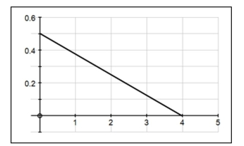a) P ( x < 1 ) b) P ( x is at least 3 ) You may need to use the following area formulas in your calculations: Area of a rectangle: A = l w Area of a trapezoid: A = \frac { 1 } { 2 } h \left( b _ { 1 } + b _ { 2 } \right) Area of a right triangle: A = \frac { 1 } { 2 } a b$ a) $P ( x < 1 )$ b) $P ( x$ is at least $3 )$ You may need to use the following area formulas in your calculations: Area of a rectangle: $A = l w$ Area of a trapezoid: $A = \frac { 1 } { 2 } h \left( b _ { 1 } + b _ { 2 } \right)$ Area of a right triangle: $A = \frac { 1 } { 2 } a b$

(Essay)

4.8/5

(38)

Question 20

Showing 1 - 20 of 57

$\text { For a discrete random variable, } \sigma _ { x } = \sum _ { x \text { values } } \left( x - \mu _ { x } \right) \cdot p ( x )$

Let $z$ denote a random variable having a standard normal distribution. Determine each of the following probabilities. a) $P ( z < 1.36 )$ b) $P ( z < - 2.05 )$ c) $P ( z > - 1.15 )$ d) $P ( - 1.10 < z < 2.54 )$

A random variable is discrete if its value depends upon the outcome of a chance experiment.

The probability that in a sequence of independent trials, each with equal probability of success, $p$ , the first success at trial $x$ is: $p ^ { x - 1 } ( 1 - p )$ .

For a continuous random variable x, the area under the density curve above an interval a to b represents the probability that the value of x is between a and b.

A normal probability plot suggests that a normal probability model is plausible if there is no obvious pattern in the scatter of points.

For every random variable, both discrete and continuous, $P ( a \leq x \leq b ) = P ( a < x < b ) \text {. }$

The number of copies sold of a newsmagazine varies from week to week. Empirical data gathered over many years suggest the following distribution of x = weekly sales (rounded to the nearest million.) What is the mean of this distribution? x 0 1 2 3 P(x) 0.15 0.25 0.40 0.20

Collecting Data in Reasonable Ways

Graphical Methods for Describing Data Distributions

Numerical Methods for Describing Data Distributions

Describing Bivariate Numerical Data

Probability

Selecting an Appropriate Method

Sampling Variability Sampling

Estimation Using a Single Sample

Asking and Answering Questions About a Population Proportion

Asking and Answering Questions About the Difference Between Two Population Proportions

Asking and Answering Questions About a Population Mean

Asking and Answering Questions About the Difference Between Two Means

Learning From Experiment Data

Filters

Exam 6: Random Variables and Probability Distributions

For a discrete random variable, σx=∑x values (x−μx)⋅p(x)\text { For a discrete random variable, } \sigma _ { x } = \sum _ { x \text { values } } \left( x - \mu _ { x } \right) \cdot p ( x ) For a discrete random variable, σx​=∑x values ​(x−μx​)⋅p(x)

A random variable is discrete if its value depends upon the outcome of a chance experiment.

The probability that in a sequence of independent trials, each with equal probability of success, ppp , the first success at trial xxx is: px−1(1−p)p ^ { x - 1 } ( 1 - p )px−1(1−p) .

For a continuous random variable x, the area under the density curve above an interval a to b represents the probability that the value of x is between a and b.

A normal probability plot suggests that a normal probability model is plausible if there is no obvious pattern in the scatter of points.

For every random variable, both discrete and continuous, P(a≤x≤b)=P(a<x<b). P ( a \leq x \leq b ) = P ( a < x < b ) \text {. }P(a≤x≤b)=P(a<x<b).

The number of copies sold of a newsmagazine varies from week to week. Empirical data gathered over many years suggest the following distribution of x = weekly sales (rounded to the nearest million.) What is the mean of this distribution? x 0 1 2 3 P(x) 0.15 0.25 0.40 0.20

Collecting Data in Reasonable Ways

Graphical Methods for Describing Data Distributions

Numerical Methods for Describing Data Distributions

Describing Bivariate Numerical Data

Probability

Selecting an Appropriate Method

Sampling Variability Sampling

Estimation Using a Single Sample

Asking and Answering Questions About a Population Proportion

Asking and Answering Questions About the Difference Between Two Population Proportions

Asking and Answering Questions About a Population Mean

Asking and Answering Questions About the Difference Between Two Means

Learning From Experiment Data

Filters

$\text { For a discrete random variable, } \sigma _ { x } = \sum _ { x \text { values } } \left( x - \mu _ { x } \right) \cdot p ( x )$

The probability that in a sequence of independent trials, each with equal probability of success, $p$ , the first success at trial $x$ is: $p ^ { x - 1 } ( 1 - p )$ .

For every random variable, both discrete and continuous, $P ( a \leq x \leq b ) = P ( a < x < b ) \text {. }$