Exam 4: Describing Bivariate Numerical Data

As early as 3 years of age, children begin to show preferences for playing with members of their own sex, and report having more same-sex than opposite-sex friends. Researchers believe that this may be the result of perceived differences in personality. In a study of 3rd and 4th graders' views on a number personality traits, children were asked to rate on a "5-point" scale: $- 2 =$ "someone possessing that trait is probably a boy" $- 1 =$ "someone possessing that trait might be a boy" $0 =$ "can't tell" $1 =$ "someone possessing that trait might be a girl" 2 = "someone possessing that trait is probably a girl" A scatterplot of the data is presented below. A single point represents the (average girls' rating, average boys' rating) for a given trait. 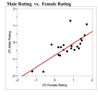Linear Fit MRating $= - 0.765 + 0.714$ FRating Summary of Fit RSquare 0.552 RSquare Adj 0.529 0.490 Analysis of Variance Source DF SS MS F Ratio Model 1 5.63 5.63 23.45 Error 19 4.56 0.24 Prob > F C. Total 20 10.20 0.0001 a) Circle the single point which represents the most influential observation. What aspect of this point makes it the most influential? b) Suppose a personality trait similar to those used in the survey was given an average of 0.0 ("can't tell") by the girls. The predicted boys' average rating would be closest to which of the 5 categories described above? c) The traits plotted above are those the researchers believe are "positive" traits, such as "mature," "honest," and "polite." The researchers thought that on average girls would rate these positive traits as characteristic of girls to a greater extent than boys would. What aspects of the plot and/or regression analysis presented above are consistent with this thinking?

What is the best fit line using the transformed data?

The coefficient of determination is equal to the positive square root of the correlation coefficient, r.

Generally, a relatively small value of $r ^ { 2 }$ is associated with a relatively small $s _ { e }$ .

A large value of $r ^ { 2 }$ indicates strong evidence for a causal relationship between $x$ and $y$ .

The Des Moines Register reported the ratings of high school sportsmanship as compiled by the Iowa High School Athletic Association. The participants and coaches from each school were rated by referees. (1 = superior, 5 = unsatisfactory.) A regression analysis of data on the average scores given to football players and coaches is shown below. 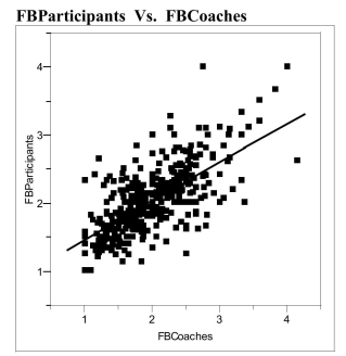Linear Fit FBParticipants $= 0.902 + 0.568$ FBCoaches Summary of Fit RSquare 0.452 RSquare Adj 0.450 0.355 Analysis of Variance Source DF SS MS F Ratio Model 1 37.505 37.505 298.2723 Error 362 45.518 0.126 Prob > F C. Total 363 83.022 <.0001 a) Interpret the value of the correlation between the ratings of coaches and participants. b) Interpret the value of the coefficient of determination. c) Interpret the value of the standard deviation about the least squares line.

The breeding success of ground-nesting birds in high altitudes can be affected by the depth of winter snow. The plot below relates the Spring percentage of White-tailed Ptarmigan hens hatching at least one egg, to the amount of snowfall in the Sierra Nevada mountain range the previous Winter. 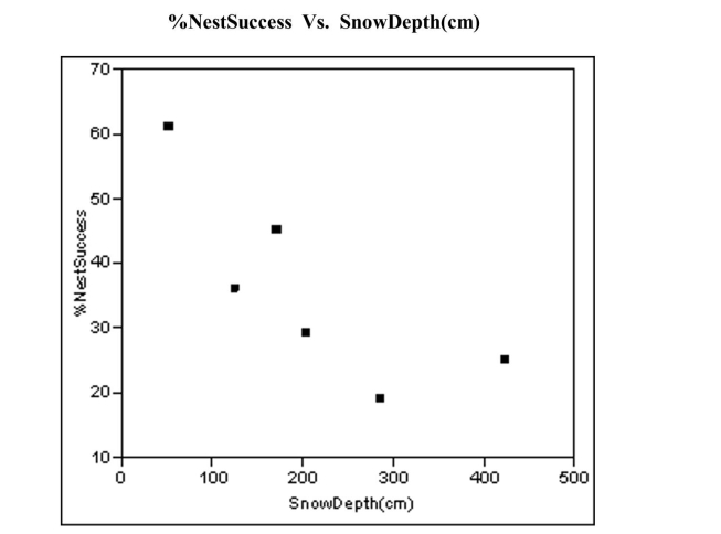a) The least sq uares line is $\% \text { NestSuccess } = 55.1816 - 0.092 ( \text { SnowDepth } )$ Graph this line on the scatterplot above. b) The least squares line is the line that minimizes the sum of the squared residuals. Using your line in part (a), graphically represent the residual associated with the snow depth of 50 cm on the scatterplot.

Assessing the "goodness" of a regression line involves considering several aspects of the fit. Consider the characteristics below. How does each contribute to an assessment of fit? That is, for each characteristic, what about the given characteristic would indicate that the regression line is "good"? a) The shape of the scatter plot b) The correlation coefficient c) The standard deviation of the residuals d) The coefficient of determination

Early humans were similar in shape to most modern large primates. The data below are average male hind limb and forelimb lengths for different species of early hominids (humans and their ancestors.) Hind limb and Forelimb lengths Hind limb Length (mm) Forelimb Length () 471 458 361 514 399 581 557 739 553 553 574 614 857 595 698 762 a) What is the value of the correlation coefficient for these data? b) What is the equation of the least squares line describing the relationship between $x =$ hind limb length and $y =$ forelimb length. c) Suppose these species are representative of all species of early human ancestors. If a new homonin species dating from about the same time were to be discovered with an average hind limb length of 500 mm, what would you predict to be the average forelimb length of this species?

One of the properties of Pearson's r is: "The value of r does not depend on which of the two variables is labeled as x." In your own words, what does this mean?

life without their physical capture and handling. In a recent study of bobcat (Lynx rufus) abundance, camera traps were placed at varying distances from a road. The data on trapping success from 8 trapping stations are presented in the table at right. The trapping success is Remote camera trapping is used to detect and monitor elusive wild- Distance (m) Trap Success 115 2.0 326 1.6 528 2.0 979 1.7 1252 1.9 1252 4.6 1459 5.7 2145 5.4 defined as the number of captures per 100 trap-nights. -Hemorrhagic disease in white-tailed deer is caused by a virus known as EHD. Immunity is given to fawns by transfer of EHD antibodies from the mother. In a study to determine how long the maternal antibodies last, blood samples were taken from a large sample of fawns of varying ages. The mean levels of EHD antibody concentration and the associated ages of fawns are given in the table below. 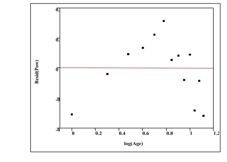After using the data to fit a straight line model, Eˆ = a + bW , significant curvature was detected in the residual plot. Two nonlinear models were chosen for further analysis, the exponential and the power models. (For these data, common logs were used to perform the transformations.) The computer output for these models is given below, and the residual plots are on the next page. $\widehat{\log E}=a+b W$ (Exponential) Bivariate Fit of LogE By Age $\log E=1.694-0.076$ Age Summary of Fit RSquare 0.975 RSquare Adj 0.973 St. Dev. Of Residuals 0.049 $\widehat{\log E}=a+b \log W$ (Power) Bivariate Fit of LogE By LogAge $\log E=1.694-0.076$ LogAge Summary of Fit RSquare 0.889 RSquare Adj 0.879 St. Dev. Of Residuals 0.105 Fawn data W=Age (Weeks) E=Mean EHDV Conc. 1 45 2 34 3 28 4 23 5 21 6 20 7 13 8 12 9 9 10 10 11 6 12 7 13 5 Residual Plots $\widehat { \log E } = a + b W$ Residual Plot - Exponential Model 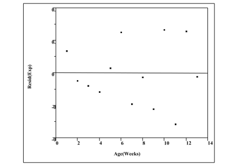$\widehat { \log E } = a + b \log W$ Residual Plot - Power Model a) For the exponential model, calculate the predicted logarithm of the EHD antibody concentration for an age of 5 weeks. b) Generally speaking, which of the two models, power or exponential, is a better choice for predicting the logarithm of the EHD antibody concentration? Provide statistical justification for your choice based on both the residual plot and the numerical summary statistics above. c) The researchers want use their model to predict EHD antibody concentrations for fawns up to 24 weeks of age. Do you think this would be reasonable? Explain why or why not.

Assessing the "goodness" of a regression line involves considering several aspects of the fit. Consider the characteristics below. How does each contribute to an assessment of fit? That is, for each characteristic, what about the given characteristic would indicate that the regression line is "good"? a) The shape of the residual plot b) The correlation coefficient c) The existence of outliers d) The coefficient of determination

What is it that the correlation coefficient measures?

The slope of the least squares line for predicting y from x and the slope of the least squares line for predicting x from y are equal.

The data below were gathered on a random sample of 7 male banded black-footed albatrosses of known age. In an effort to monitor diseases of these animals, biologists would like to be able to estimate the lifespan of healthy albatrosses in the larger population. In males of this species gonad size (the size of the sex gland) is associated with age. Gonad size vs. Age in Black-footed albatrosses Gonad Size (sq mm) Age (Years) 42 1.42 60 4.75 20 0.67 96 23.64 24 0.52 27 2.35 27 1.4 a) What is the value of the correlation coefficient for these data? b) What is the equation of the least squares line describing the relationship between $x =$ Gonad Size and $y =$ Age. c) If these albatrosses are representative of the population of all albatrosses, what would you predict to be the age of a male albatross with a gonad size of $50 \mathrm { sq }$ . mm? Show any calculations below. d) The largest albatross gonad size in the sample, $96 \mathrm { sq } \mathrm { mm }$ , is associated with an age of $23.64$ years. These animals are thought to live for up to 40 years. Would it be reasonable to use the equation from part (b) above to predict the age for an albatross with a gonad size of $150 \mathrm { sq } \mathrm { mm }$ ? Why or why not?

a) What is the equation of the least-squares line for predicting tenacity using amino b) Graph the least squares best fit line on the scatter plot that appears on the next page. acid ratio Amino acid ratio and tenacity for linings for 16 Japanese kimonos Amino acid ratio Tenacity 2.05 1.20 1.78 1.60 2.08 1.30 2.62 0.90 2.00 1.80 1.92 1.60 1.89 1.20 1.32 2.40 1.20 3.10 1.63 2.80 1.05 4.40 1.60 3.00 1.60 2.10 1.98 3.10 2.16 1.40 2.10 1.90 c) Approximately what proportion of the variability in tenacity is explained by the linear relationship between tenacity and the amino acid ratio? The theory of fiber strength suggests that the relationship between fiber tenacity and amino acid ratio is logarithmic, i.e. $\hat { T } = \alpha + \beta \log ( R )$ , where $T$ is the tenacity and $R$ is the amino acid ratio. Perform the appropriate transformation of variable(s) and fit this logarithmic model to the data. 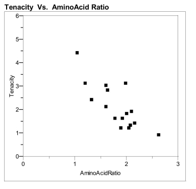protein and biodegradable. It would be beneficial to be able to assess the delicacy of a fabric before making decisions about displaying it in a museum. Chemical analysis might give some evidence about the brittle nature of a fabric. Bio- chemical data were acquired from the linings of Some delicate fabrics are natural silks, made of sixteen 19th and early 20th century Japanese kimonos. Investigators measured the concentration of certain amino acids ("Amino acid ratio") as well as the breaking stress ("tenacity") of the 16 kimono fabrics.

The correlation coefficient, r, does not depend on the units of measurement of the two variables.

The study of prehistoric birds depends on imprints of a prehistoric creature's remains in stone, commonly known as fossils. To study ancient ecosystems effectively it would be useful know the actual mass of individual birds, but this information is not preserved in the fossil record. It seems reasonable that the biomechanics of birds is much the same today as in the past. For example, today's relationship between the wing length and total weight of a bird should be very similar to that for birds from the distant past. The wing lengths of ancient birds are readily obtainable from the fossil record, but the weight is not. A regression model expressing the relationship between wing length and total weight of modern birds could be used to estimate the mass of similar prehistoric birds. Data for some species of modern birds of prey and are given below. Wing length and total weight of modern species of birds of prey Bird species Wing length () Total weight (kilograms) Gyps fulvus 69.8 7.27 Gypaetus barbatus grandis 71.7 5.39 Catharista atrata 50.2 1.70 Aguila chrysatus 68.2 3.71 Hieraeus fasciatus 56.0 2.06 Helotarsus ecaudatus 51.2 2.10 Geranoatus melanoleucus 51.5 2.12 Circatus gallicus 53.3 1.66 Buteo bueto 40.4 1.03 Pernis apivorus 45.1 0.62 Pandion haliatus 49.6 1.11 Circus aeruginosos 41.3 0.68 Circus cyaneus (female) 37.4 0.472 Circus cyaneus (male) 33.9 0.331 Circus pygargus 35.9 0.237 Circus macrurus 35.7 0.386 Milvus milvus 50.7 0.927 -Investigators would like to model the relationship between Wing Length and Weight. The least squares line for predicting total weight using wing length as a predictor is of interest. a) What is the equation of the least-squares line? b) Graph the least-squares line on the scatter plot below. c) Approximately what proportion of the variability in weight is explained by the wing length?

life without their physical capture and handling. In a recent study of bobcat (Lynx rufus) abundance, camera traps were placed at varying distances from a road. The data on trapping success from 8 trapping stations are presented in the table at right. The trapping success is Remote camera trapping is used to detect and monitor elusive wild- Distance (m) Trap Success 115 2.0 326 1.6 528 2.0 979 1.7 1252 1.9 1252 4.6 1459 5.7 2145 5.4 defined as the number of captures per 100 trap-nights. -a) What is the least squares line for predicting trap success using the distance from the road? b) Sketch the least squares line on the scatter plot. c) What is the value of $r ^ { 2 } ?$ Interpret this value in the context of this problem. 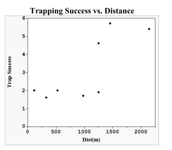d) One of the trap sites is 1459 meters from the road. Calculate the residual for this trap site. e) Suppose that the trap sites you analyzed above are representative of the population of all trap sites. In general, do you think the linear model is a good model for these data? Justify your answer by appealing to the scatterplot and other summary statistics.

As early as 3 years of age, children begin to show preferences for playing with members of their own sex, and report having more same-sex than opposite-sex friends. Researchers believe that this may be the result of perceived differences in personality. In a study of 3rd and 4th graders' views on a number personality traits, children were asked to rate on a "5-point" scale: $- 2 =$ "someone possessing that trait is probably a boy" $- 1 =$ "someone possessing that trait might be a boy" $0 =$ "can't tell" $1 =$ "someone possessing that trait might be a girl" $2 =$ "someone possessing that trait is probably a girl" A scatterplot of the data is presented below. A single point represents the (average girls' rating, average boys' rating) for a given trait. 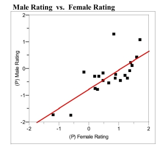Male Rating vs. Female Rating Linear Fit MRating =-0.765+0.714 FRating Summary of Fit RSquare 0.552 RSquare Adj 0.529 s 0.490 Analysis of Variance Source DF SS MS F Ratio Model 1 5.63 5.63 23.45 Error 19 4.56 0.24 Prob > C. Total 20 10.20 0.0001 a) Circle the single point that represents the most influential observation. What aspect of this point makes it the most influential? b) Suppose a personality trait similar to those used in the survey was given an average of 0.0 ("can't tell") by the girls. The predicted boys' average rating would be closest to which of the 5 categories described above? c) The traits plotted above are those the researchers believe are "positive" traits, such as "mature," "honest," and "polite." The researchers thought that on average girls would rate these positive traits as characteristic of girls to a greater extent than boys would. What aspects of the plot and/or regression analysis presented above are consistent with this thinking?