Exam 16: Multiple Regression
Exam 1: What Is Statistics17 Questions
Exam 2: Types of Data, Data Collection and Sampling18 Questions
Exam 3: Graphical Descriptive Techniques Nominal Data17 Questions
Exam 4: Graphical Descriptive Techniques Numerical Data65 Questions
Exam 5: Numerical Descriptive Measures149 Questions
Exam 6: Probability113 Questions
Exam 7: Random Variables and Discrete Probability Distributions50 Questions
Exam 8: Continuous Probability Distributions113 Questions
Exam 9: Statistical Inference and Sampling Distributions69 Questions
Exam 10: Estimation: Describing a Single Population125 Questions
Exam 11: Estimation: Comparing Two Populations36 Questions
Exam 12: Hypothesis Testing: Describing a Single Population124 Questions
Exam 13: Hypothesis Testing: Comparing Two Populations69 Questions
Exam 14: Additional Tests for Nominal Data: Chi-Squared Tests113 Questions
Exam 15: Simple Linear Regression and Correlation213 Questions
Exam 16: Multiple Regression122 Questions
Exam 17: Time-Series Analysis and Forecasting147 Questions
Exam 18: Index Numbers27 Questions
Select questions type
In regression analysis, the total variation in the dependent variable y, measured by , can be decomposed into two parts: the explained variation, measured by SSR, and the unexplained variation, measured by SSE.
(True/False)
4.9/5  (28)
(28)
Multicollinearity is a situation in which the independent variables are highly correlated with the dependent variable.
(True/False)
4.8/5 (37)
A statistics professor investigated some of the factors that affect an individual student's final grade in his or her course. He proposed the multiple regression model: .
Where:
y = final mark (out of 100). = number of lectures skipped. = number of late assignments. = mid-term test mark (out of 100).
The professor recorded the data for 50 randomly selected students. The computer output is shown below.
THE REGRESSION EQUATION IS
ŷ = Predictor Coef StDev Constant 41.6 17.8 2.337 -3.18 1.66 -1.916 -1.17 1.13 -1.035 0.63 0.13 4.846 se = 13.74, R2 = 30.0%. ANALYSIS OF VARIANCE Source of Variation SS MS F Regression 3 3716 1238.667 6.558 Error 46 8688 188.870 Total 49 12404 Do these data provide enough evidence at the 1% significance level to conclude that the final mark and the mid-term mark are positively linearly related?
(Essay)
4.9/5 (29)
Test the hypotheses: There is no first-order autocorrelation
HA : There is first-order autocorrelation,
given that the Durbin-Watson statistic d = 1.89, n = 28, k = 3 and 0.05.
(Essay)
4.8/5 (28)
A statistician wanted to determine whether the demographic variables of age, education and income influence the number of hours of television watched per week. A random sample of 25 adults was selected to estimate the multiple regression model .
Where:
y = number of hours of television watched last week. = age. = number of years of education. = income (in $1000s).
The computer output is shown below.
THE REGRESSION EQUATION IS
ŷ = Predictor Coef StDev Constant 22.3 10.7 2.084 0.41 0.19 2.158 -0.29 0.13 -2.231 -0.12 0.03 -4.00 se = 4.51 R2 = 34.8%. ANALYSIS OF VARIANCE Source of Variation SS MS F Regression 3 227 75.667 3.730 Error 21 426 20.286 Total 24 653 Interpret the coefficient .
(Essay)
4.8/5 (36)
Pop-up coffee vendors have been popular in the city of Adelaide in 2013. A vendor is interested in knowing how temperature (in degrees Celsius) and number of different pastries and biscuits offered to customers impacts daily hot coffee sales revenue (in $00's).
A random sample of 6 days was taken, with the daily hot coffee sales revenue and the corresponding temperature and number of different pastries and biscuits offered on that day, noted.
Excel output for a multiple linear regression is given below: Coffee sales revenue Temperature Pastries/biscuits 6.5 25 7 10 17 13 5.5 30 5 4.5 35 6 3.5 40 3 28 9 15 SUMMARY OUTPUT Regression Statistios Multiple R 0.87 R Square 0.75 Adjusted R Square 0.59 Standard Error 5.95 Observations 6.00 ANOVA df SS MS F Significance F Regression 2.00 322.14 161.07 4.55 0.12 Residual 3.00 106.20 35.40 Total 5.00 428.33 Coeffients Standard Error tStat P-value Lower 95\% Upper 95\% Intercept 18.68 37.88 0.49 0.66 -101.88 139.24 Temperature -0.50 0.83 -0.60 0.59 -3.15 2.15 Pastries/biscuits 0.49 2.02 0.24 0.82 -5.94 6.92 Test the significance of the overall regression model, at α of 5%.
(Essay)
4.7/5 (24)
Pop-up coffee vendors have been popular in the city of Adelaide in 2013. A vendor is interested in knowing how temperature (in degrees Celsius) and number of different pastries and biscuits offered to customers impacts daily hot coffee sales revenue (in $00's).
A random sample of 6 days was taken, with the daily hot coffee sales revenue and the corresponding temperature and number of different pastries and biscuits offered on that day, noted.
Describe the following scatterplots. 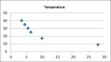 Scatterplot of Daily hot coffee sales revenue vs Temperature
 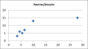 Scatterplot of Daily hot coffee sales revenue Pastries/biscuits
 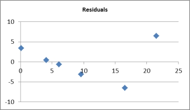 Residual scatterplot of Daily hot coffee sales revenue vs fitted values
(Essay)
4.9/5 (22)
An actuary wanted to develop a model to predict how long individuals will live. After consulting a number of physicians, she collected the age at death (y), the average number of hours of exercise per week ( ), the cholesterol level ( ), and the number of points by which the individual's blood pressure exceeded the recommended value ( ). A random sample of 40 individuals was selected. The computer output of the multiple regression model is shown below:
THE REGRESSION EQUATION IS
ŷ = Predictor Coef StDev Constant 55.8 11.8 4.729 1.79 0.44 4.068 -0.021 0.011 -1.909 -0.016 0.014 -1.143 se = 9.47 R2 = 22.5%. ANALYSIS OF VARIANCE Source olf Variation df SS MS F Regression 3 936 312 3.477 Error 36 3230 89.722 Total 39 4166 Interpret the coefficient .
(Essay)
4.9/5 (36)
For the estimated multiple regression model ŷ = 30 4x1 + 5x2 +3 x3, a one unit increase in x3, holding x1 and x2 constant, will result in which of the following changes in y?
(Multiple Choice)
4.9/5 (35)
An actuary wanted to develop a model to predict how long individuals will live. After consulting a number of physicians, she collected the age at death (y), the average number of hours of exercise per week ( ), the cholesterol level ( ), and the number of points by which the individual's blood pressure exceeded the recommended value ( ). A random sample of 40 individuals was selected. The computer output of the multiple regression model is shown below:
THE REGRESSION EQUATION IS
ŷ = Predictor Coef StDev Constant 55.8 11.8 4.729 1.79 0.44 4.068 -0.021 0.011 -1.909 -0.016 0.014 -1.143 se = 9.47 R2 = 22.5%. ANALYSIS OF VARIANCE Source of Variation SS MS F Regression 3 936 312 3.477 Error 36 3230 89.722 Total 39 4166 Is there enough evidence at the 10% significance level to infer that the model is useful in predicting length of life?
(Essay)
4.9/5 (36)
For a set of 30 data points, Excel has found the estimated multiple regression equation to be = ?8.61 + 22x1 + 7x2 + 28x3, and has listed the t statistic for testing the significance of each regression coefficient. Using the 5% significance level for testing whether ?3 = 0, the critical region will be that the absolute value of the t statistic for ?3 is greater than or equal to:
(Multiple Choice)
5.0/5 (42)
In multiple regression, because of a commonly occurring problem called multicollinearity, the
t-tests of the individual coefficients may indicate that some independent variables are not linearly related to the dependent variable, when in fact they are.
(True/False)
4.8/5 (33)
An economist wanted to develop a multiple regression model to enable him to predict the annual family expenditure on clothes. After some consideration, he developed the multiple regression model: .
Where:
y = annual family clothes expenditure (in $1000s) = annual household income (in $1000s) = number of family members = number of children under 10 years of age
The computer output is shown below.
THE REGRESSION EQUATION IS
ŷ = Predictor Coef StDev Constant 1.74 0.630 2.762 0.091 0.025 3.640 0.93 0.290 3.207 0.26 0.180 1.444 se = 2.06, R2 = 59.6%. ANALYSIS OF VARIANCE Source of Variation SS MS F Regression 3 288 96 22.647 Error 46 195 4.239 Total 49 483 Test at the 10% significance level to determine whether annual household income and annual family clothes expenditure are linearly related.
(Essay)
4.9/5 (28)
Which of the following is used to test the significance of the overall regression equation?
(Multiple Choice)
4.8/5 (41)
An economist wanted to develop a multiple regression model to enable him to predict the annual family expenditure on clothes. After some consideration, he developed the multiple regression model: .
Where:
y = annual family clothes expenditure (in $1000s) = annual household income (in $1000s) = number of family members = number of children under 10 years of age
The computer output is shown below.
THE REGRESSION EQUATION IS
ŷ = Predictor Coef StDev Constant 1.74 0.630 2.762 0.091 0.025 3.640 0.93 0.290 3.207 0.26 0.180 1.444 se = 2.06, R2 = 59.6%.. ANALYSIS OF VARIANCE Source of Variation SS MS F Regression 3 288 96 22.647 Error 46 195 4.239 Total 49 483 Interpret the coefficient .
(Essay)
4.8/5 (28)
An economist wanted to develop a multiple regression model to enable him to predict the annual family expenditure on clothes. After some consideration, he developed the multiple regression model: .
Where:
y = annual family clothes expenditure (in $1000s) = annual household income (in $1000s) = number of family members = number of children under 10 years of age
The computer output is shown below.
THE REGRESSION EQUATION IS
ŷ = Predictor Coef StDev Constant 1.74 0.630 2.762 0.091 0.025 3.640 0.93 0.290 3.207 0.26 0.180 1.444 se = 2.06, R2 = 59.6%. ANALYSIS OF VARIANCE Source of Variation SS MS F Regression 3 288 96 22.647 Error 46 195 4.239 Total 49 483 Test the overall model's validity at the 5% significance level.
(Essay)
4.8/5 (26)
A multiple regression analysis that includes 4 independent variables results in a sum of squares for regression of 1200 and a sum of squares for error of 800. The coefficient of determination will be:
(Multiple Choice)
4.9/5 (26)
Which of the following best describes the range of the coefficient of determination?
(Multiple Choice)
4.8/5 (38)
A statistician estimated the multiple regression model , with 45 observations. The computer output is shown below. However, because of a printer malfunction, some of the results are not shown. These are indicated by the boldface letters a to l. Fill in the missing results (up to three decimal places). Predictor Coef StDev t Constant 2.794 a 6.404 b 0.007 -0.025 0.383 0.072 c se = d R2 = e. ANALYSIS OF VARIANCE Source of Variation df SS MS F Regression f i j l Error g 11.884 k Total h 26.887
(Essay)
4.8/5 (41)
Filters
- Essay(0)
- Multiple Choice(0)
- Short Answer(0)
- True False(0)
- Matching(0)