Exam 10: Regression With Panel Data
With Panel Data, regression software typically uses an "entity-demeaned" algorithm because
C
The notation for panel data is (Xit, Yit), i = 1, ..., n and t = 1, ..., T because
C
A researcher investigating the determinants of crime in the United Kingdom has data for 42 police regions over 22 years. She estimates by OLS the following regression
ln(cmrt)it = ?i + ?t + ?1unrtmit + ?2proythit + ?3 ln(pp)it + uit; i = 1,..., t = 1,..., 22
where cmrt is the crime rate per head of population, unrtm is the unemployment rate of males, proyth is the proportion of youths, pp is the probability of punishment measured as (number of convictions)/(number of crimes reported). ? and ? are area and year fixed effects, where ?i equals one for area i and is zero otherwise for all i, and ?t is one in year t and zero for all other years for t = 2, …, 22. ?1 is not included.
(a)What is the purpose of excluding ?1? What are the terms ? and ? likely to pick up? Discuss the advantages of using panel data for this type of investigation.
(b)Estimation by OLS using heteroskedasticity and autocorrelation-consistent standard errors results in the following output, where the coefficients of the fixed effects are not reported:
(0.109) (0.179) (0.024)
Comment on the results. In particular, what is the effect of a ten percent increase in the probability of punishment?
(c)To test for the relevance of the area fixed effects, your restrict the regression by dropping all entity fixed effects and add single constant is added. The relevant F-statistic is 135.28. What are the degrees of freedom? What is the critical value from your F table?
(d)Although the test rejects the hypothesis of eliminating the fixed effects from the regression, you want to analyze what happens to the coefficients and their standard errors when the equation is re-estimated without fixed effects. In the resulting regression, and do not change by much, although their standard errors roughly double. However, is now 1.340 with a standard error of 0.234. Why do you think that is?
(a)Since there is no constant in addition to the entity and time fixed effects, setting φt to one in year t and zero for all other years for t = 1, …, 22 would result in perfect multicollinearity. α picks up omitted variables that are specific to police regions and do not vary over time. φ picks up effects that are common to all police regions in a given year. Attitudes toward crime may vary between rural regions and metropolitan areas. These would be hard to capture through measurable variables. Common macroeconomic shocks that affect all regions equally will be captured by the time fixed effects. Although some of these variables could be explicitly introduced, the list of possible variables is long. By introducing time fixed effects, the effect is captured all in one variable.
(b)A higher male unemployment rate and a higher proportion of youths increase the crime rate, while a higher probability of punishment decreases the crime rate. The coefficients on the probability of punishment and the proportion of youths is statistically significant, while the male unemployment rate is not. The regression explains roughly 90 percent of the variation in crime rates in the sample. A ten percent increase in the number of convictions over the number of crimes reported decreases the crime rate by roughly six percent.
(c)The coefficients of the three regressors other than the entity coefficients would have been unaffected, had there been a constant in the regression and (n-1)police region specific entity variables. In this case, the entity coefficients on the police regions would have indicated deviations from the constant for the first police region. Hence there are 41 restrictions imposed by eliminating the entity fixed effects and adding a constant. Since there are over 100 observations (900 degrees of freedom), the critical value for F41,∞ ≈ F30,∞ = 1.70 at the 1% level. Hence the restrictions are rejected.
(d)This result would make the male unemployment rate coefficient significant. It suggests that male unemployment rates change slowly over the years in a given police district and that this effect is picked up by the entity fixed effects. Of course, there are other slowly changing variables, such as attitudes towards crime, that are captured by these fixed effects.
Consider estimating the effect of the beer tax on the fatality rate, using time and state fixed effect for the Northeast Region of the United States (Maine, Vermont, New Hampshire, Massachusetts, Connecticut and Rhode Island)for the period 1991-2001. If Beer Tax was the only explanatory variable, how many coefficients would you need to estimate, excluding the constant?
Consider the following panel data regression with a single explanatory variable
Yit = β0 + β1Xit + uit.
In each of the examples below, you will be adding entity and time fixed effects. Indicate the total number of coefficients that need to be estimated.
(a)The effect of beer taxes on the fatality rate, annual data, 1982-1988, nine U.S. regions (New England, Pacific, Mid-Atlantic, East North Central, etc.).
(b)The effect of the minimum wage on teenage employment, annual data, 1963-2000, five Canadian Regions (Atlantic Provinces, Quebec, Ontario, Prairies, British Columbia).
(c)The effect of savings rates on per capita income, data for three decades (1960-1969, 1970-1979, 1980-1989; one observation per decade), 104 countries of the world.
(d)The effect of pitching quality in baseball (as measured by the Team ERA)on the winning percentage, annual data, 1998-1999 season, 1999-2000 season, 30 teams.
A study, published in 1993, used U.S. state panel data to investigate the relationship between minimum wages and employment of teenagers. The sample period was 1977 to 1989 for all 50 states. The author estimated a model of the following type: where E is the employment to population ratio of teenagers, M is the nominal minimum wage, and W is average hourly earnings in manufacturing. In addition, other explanatory variables, such as the adult unemployment rate, the teenage population share, and the teenage enrollment rate in school, were included.
(a)Name some of the factors that might be picked up by time and state fixed effects.
(b)The author decided to use eight regional dummy variables instead of the 49 state dummy variables. What is the implicit assumption made by the author? Could you test for its validity? How?
(c)The results, using time and region fixed effects only, were as follows: = -0.182 × ln(Mit /Wit )+ ...; R2= 0.727
(0.036)
Interpret the result briefly.
(d)State minimum wages do not exceed federal minimum wages often. As a result, the author decided to choose the federal minimum wage in his specification above. How does this change your interpretation? How is the original equation affected by this?
A pattern in the coefficients of the time fixed effects binary variables may reveal the following in a study of the determinants of state unemployment rates using panel data:
Assume that for the T = 2 time periods case, you have estimated a simple regression in changes model and found a statistically significant positive intercept. This implies
You learned in intermediate macroeconomics that certain macroeconomic growth models predict conditional convergence or a catch up effect in per capita GDP between the countries of the world. That is, countries which are further behind initially in per-capita GDP will grow faster than the leader. You gather data from the Penn World Tables to test this theory.
(a)By limiting your sample to 24 OECD countries, you hope to have a more homogeneous set of countries in your sample, i.e., countries that are not too different with respect to their institutions. To simplify matters, you decide to only test for unconditional convergence. In that case, the laggards catch up even without taking into account differences in some of the driving variables. Your scatter plot and regression for the time period 1975-1989 are as follows: 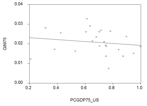 = 0.024 - 0.005 PCGDP75_US; R2= 0.025, SER = 0.006
(0.06)(0.008)
where is the average annual growth rate of per capita GDP from 1975-1989, and PCGDP75_US is per capita GDP relative to the United States in 1975. Numbers in parenthesis are heteroskedasticity-robust standard errors.
Interpret the results. Is there indication of unconditional convergence? What critical value did you use?
(b)Although you are quite discouraged by the result, you think that it might be due to the specific time period used. During this period, there were two OPEC oil price shocks with varying degrees of exposure for the OECD countries. You therefore repeat the exercise for the period 1960-1974, with the following results:
= 0.024 - 0.005 PCGDP75_US; R2= 0.025, SER = 0.006
(0.06)(0.008)
where is the average annual growth rate of per capita GDP from 1975-1989, and PCGDP75_US is per capita GDP relative to the United States in 1975. Numbers in parenthesis are heteroskedasticity-robust standard errors.
Interpret the results. Is there indication of unconditional convergence? What critical value did you use?
(b)Although you are quite discouraged by the result, you think that it might be due to the specific time period used. During this period, there were two OPEC oil price shocks with varying degrees of exposure for the OECD countries. You therefore repeat the exercise for the period 1960-1974, with the following results: 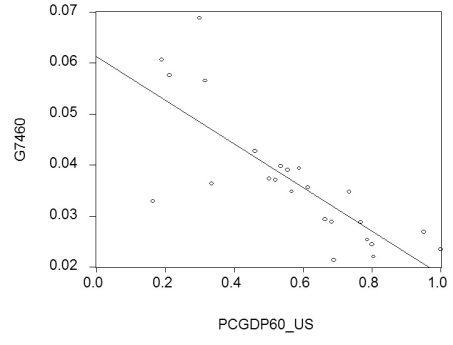 = 0.061 - 0.043 PCGDP60_US; R2= 0.613, SER = 0.008
(0.004)(0.007)
where is the average annual growth rate of per capita GDP from 1960-1974, and PCGDP60_US is per capita GDP relative to the United States in 1960.
Compare this regression to the previous one.
(c)You decide to run one more regression in differences. The dependent variable is now the change in the growth rate of per capita GDP from 1960-1974 to 1975-1989 (diffg)and the regressor the difference in the initial conditions (diffinit). This produces the following graph and regression:
= 0.061 - 0.043 PCGDP60_US; R2= 0.613, SER = 0.008
(0.004)(0.007)
where is the average annual growth rate of per capita GDP from 1960-1974, and PCGDP60_US is per capita GDP relative to the United States in 1960.
Compare this regression to the previous one.
(c)You decide to run one more regression in differences. The dependent variable is now the change in the growth rate of per capita GDP from 1960-1974 to 1975-1989 (diffg)and the regressor the difference in the initial conditions (diffinit). This produces the following graph and regression: 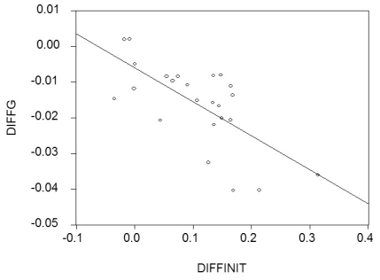 = -0.006 - 0.096 × diffinit; R2 = 0.468; SER = 0.009
(0.03)(0.021)
Interpret these results. Explain what has happened to unobservable omitted variables that are constant over time. Suggest what some of these variables might be.
(d)Given that there are only two time periods, what other methods could you have employed to generate the identical results? Why do you think that the slope coefficient in this regression is significant given the results over the sub-periods?
= -0.006 - 0.096 × diffinit; R2 = 0.468; SER = 0.009
(0.03)(0.021)
Interpret these results. Explain what has happened to unobservable omitted variables that are constant over time. Suggest what some of these variables might be.
(d)Given that there are only two time periods, what other methods could you have employed to generate the identical results? Why do you think that the slope coefficient in this regression is significant given the results over the sub-periods?
Consider the case of time fixed effects only, i.e.,
Yit = β0 + β1Xit + β3St + uit,
First replace β0 + β3St with φt. Next show the relationship between the φt and δt in the following equation
Yit = β0 + β1Xit + δ2B2t + ... + δTBTt + uit,
where each of the binary variables B2, …, BT indicates a different time period. Explain in words why the two equations are the same. Finally show why there is perfect multicollinearity if you add another binary variable B1. What is the intuition behind the fact that the OLS estimator does not exist in this case? Would that also be the case if you dropped the intercept?
Time Fixed Effects regression are useful in dealing with omitted variables
(Requires Matrix Algebra)Consider the time and entity fixed effect model with a single explanatory variable
Yit = ?0 + ?1Xit + D2i + ... + Dni + ?2B2t + ... + ?TBTt + uit,
For the case of n = 4 and T = 3, write this model in the form Y = X? + U, where, in general,
Y = , U = , X = 1 \ldots 1 \ldots 1 \ldots = , and ? = How would the X matrix change if you added two binary variables, D1 and B1? Demonstrate that in this case the columns of the X matrix are not independent. Finally show that elimination of one of the two variables is not sufficient to get rid of the multicollinearity problem. In terms of the OLS estimator, = ( X)-1
Y, why does perfect multicollinearity create a problem?
If you included both time and entity fixed effects in the regression model which includes a constant, then
When you add state fixed effects to a simple regression model for U.S. states over a certain time period, and the regression R2 increases significantly, then it is safe to assume that
In the panel regression analysis of beer taxes on traffic deaths, the estimation period is 1982-1988 for the 48 contiguous U.S. states. To test for the significance of time fixed effects, you should calculate the F-statistic and compare it to the critical value from your Fq,∞ distribution, where q equals
In the Fixed Time Effects regression model, you should exclude one of the binary variables for the time periods when an intercept is present in the equation
HAC standard errors and clustered standard errors are related as follows:
Consider the regression example from your textbook, which estimates the effect of beer taxes on fatality rates across the 48 contiguous U.S. states. If beer taxes were set nationally by the federal government rather than by the states, then
In the Fixed Effects regression model, using (n - 1)binary variables for the entities, the coefficient of the binary variable indicates
Filters
- Essay(0)
- Multiple Choice(0)
- Short Answer(0)
- True False(0)
- Matching(0)