Exam 9: Assessing Studies Based on Multiple Regression

Assume the following model of the labor market: N^d = ?₀ + ?₁ $\frac { W } { P }$ + u N^s = ?₀ + ?₁ $\frac { W } { P }$ + v N^d = N^s = N where N is employment, (W/P)is the real wage in the labor market, and u and v are determinants other than the real wage which affect labor demand and labor supply (respectively). Let E(u)= E(v)= 0; var(u)= $\sigma _ { u } ^ { 2 }$ ; var(v)= $\sigma _ { v } ^ { 2 }$ ; cov(u,v)= 0 Assume that you had collected data on employment and the real wage from a random sample of observations and estimated a regression of employment on the real wage (employment being the regressand and the real wage being the regressor). It is easy but tedious to show that $\left( \hat { \beta } _ { 1 } - \beta _ { 1 } \right) \xrightarrow{p} \left( \gamma _ { 1 } - \beta _ { 1 } \right) \frac { \sigma _ { u } ^ { 2 } } { \sigma _ { u } ^ { 2 } + \sigma _ { v } ^ { 2 } }$ > 0 since the slope of the labor supply function is positive and the slope of the labor demand function is negative. Hence, in general, you will not find the correct answer even in large samples. a. What is this bias referred to? b. What would the relationship between the variance of the labor supply/demand shift variable have to be for the bias to disappear? c. Give an intuitive answer why the bias would disappear in that situation. Draw a graph to illustrate your argument.

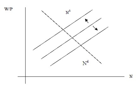
The reliability of a study using multiple regression analysis depends on all of the following with the exception of

Your textbook only analyzed the case of an error-in-variables bias of the type $\bar X$ _i= X_i + w_i. What if the error were generated in the simple regression model by entering data that always contained the same typographical error, say $\bar X$ _i= X_i + a or $\bar X$ _i= bX_i, where a and b are constants. What effect would this have on your regression model?

Comparing the California test scores to test scores in Massachusetts is appropriate for external validity if

Sample selection bias

In the simple, one-explanatory variable, errors-in-variables model, the OLS estimator for the slope is inconsistent. The textbook derived the following result $\hat { \beta } _ { 1 } \stackrel { p } { \longrightarrow } \frac { \sigma _ { X } ^ { 2 } } { \sigma _ { X } ^ { 2 } + \sigma _ { w } ^ { 2 } } \beta _ { 1 }$ Show that the OLS estimator for the intercept behaves as follows in large samples: $\hat { \beta } _ { 1 } \stackrel { p } { \rightarrow } \beta _ { 0 } + \mu \widetilde { \mathrm { X } } \frac { \sigma _ { w } ^ { 2 } } { \sigma _ { \mathrm { X } } ^ { 2 } + \sigma _ { w } ^ { 2 } } \beta _ { 1 }$ where $\bar { X }$ $\stackrel { p } { \rightarrow }$ ${ } ^ { { } ^ { \mu } } \widetilde { X }$

Possible solutions to omitted variable bias, when the omitted variable is not observed, include the following with the exception of

The true causal effect might not be the same in the population studied and the population of interest because

Your textbook gives the following example of simultaneous causality bias of a two equation system: Y_i = β₀ + β₁X_i + u_i X_i = $y _ { 0 }$ + $y _ { 1 }$ Y_i + v_i In microeconomics, you studied the demand and supply of goods in a single market. Let the demand ( $Q _ { i } ^ { D }$ )and supply ( $Q _ { i } ^ { S }$ )for the i-th good be determined as follows, $Q _ { i } ^ { D }$ = β₀ - β₁P_i + u_i, $Q _ { i } ^ { S }$ = $y _ { 0 }$ - $y _ { 1 }$ P_i + v_i, where P is the price of the good. In addition, you typically assume that the market clears. Explain how the simultaneous causality bias applies in this situation. The textbook explained a positive correlation between X_i and u_i for $y _ { 1 }$ > 0 through an argument that started from "imagine that u_i is negative." Repeat this exercise here.

The Phillips curve is a relationship in macroeconomics between the inflation rate (inf)and the unemployment rate (ur). Estimating the Phillips curve using quarterly data for the United States from 1962:I to 1995:IV, you find $\widehat{\text { Inf t}}$ = 4.08 + 0.118 ur_t, R² = 0.003, SER = 3.148 (1.11)(0.176) (a)Explain why, at first glance, this is a surprising result. (b)Do you think that there is omitted variable bias in the regression? (c)What other threats to internal validity may be present? (d)If you could find a proper specification for the Phillips curve using United States data, what external validity criteria would you suggest?

Your textbook compares the results of a regression of test scores on the student-teacher ratio using a sample of school districts from California and from Massachusetts. Before standardizing the test scores for California, you get the following regression result: $\widehat{\text { TestScr }}$ ^{= 698.9 - 2.28×STR} n = 420, R2 = 0.051, SER = 18.6 _{In addition, you are given the following information: the sample mean of the student-teacher ratio is 19.64 with a standard deviation of 1.89, and the standard deviation of the test scores is 19.05. a. After standardizing the test scores variable and running the regression again, what is the value of the slope? What is the meaning of this new slope here (interpret the result)? b. What will be the new intercept? Now that test scores have been standardized, should you interpret the intercept?} c. Does the regression R2 change between the two regressions? What about the t-statistic for the slope estimator?

Your textbook used the California Standardized Testing and Reporting (STAR)data set on test student performance in Chapters 4-7. One justification for putting second to twelfth graders through such an exercise once a year is to make schools more accountable. The hope is that schools with low scores will improve the following year and in the future. To test for the presence of such an effect, you collect data from 1,000 L.A. County schools for grade 4 scores in 1998 and 1999, both for reading (Read)and mathematics (Maths). Both are on a scale from zero to one hundred. The regression results are as follows (homoskedasticity-only standard errors in parentheses): = 6.967+0.9192=0.825, SER =7.818 (0.542)(0.013) = 4.131+0.943, Re a==0.887, SER =6.416 (0.409)(0.011) (a)Interpret the results and indicate whether or not the coefficients are significantly different from zero. Do the coefficients have the expected sign and magnitude? (b)Discuss various threats to internal and external validity, and try to assess whether or not these are likely to be present in your study. (c)Changing the estimation method to allow for heteroskedasticity-robust standard errors produces four new standard errors: (0.539), (0.015), (0.452), and (0.015)in the order of appearance in the two equations above. Given these numbers, do any of your statements in (b)change? Do you think that the coefficients themselves changed? (d)If reading and maths scores were the same in 1999 as in 1998, on average, what coefficients would you expect for the intercept and the slope? How would you test for the restrictions? (e)The appropriate F-statistic in (d)is 138.27 for the maths scores, and 104.85 for the reading scores. Comparing these values to the critical values in the F table, can you reject the null hypothesis in each case? (f)Your professor tells you that the analysis reminds her of "Galton's Fallacy." Sir Francis Galton regressed the height of children on the average height of their parents. He found a positive intercept and a slope between zero and one. Being concerned about the height of the English aristocracy, he interpreted the results as "regression to mediocrity" (hence the name regression). Do you see the parallel?

A possible solution to errors-in-variables bias is to

Applying the analysis from the California test scores to another U.S. state is an example of looking for

You have decided to analyze the year-to-year variation in temperature data. Specifically you want to use this year's temperature to predict next year's temperature for certain cities. As a result, you collect the daily high temperature (Temp)for 100 randomly selected days in a given year for three United States cities: Boston, Chicago, and Los Angeles. You then repeat the exercise for the following year. The regression results are as follows (heteroskedasticity-robust standard errors in parentheses): $\widehat { \operatorname { Temp } _ { t } ^ { B O S } } = 18.19 + 0.75 \times \operatorname { Temp } _ { t - 1 } ^ { B O S } ; R ^ { 2 } = 0.62$ , SER $= 12.33$ $\quad$$\quad$$\quad$$\quad$$\quad$ (6.46) $( 0.10 )$ $\widehat { \text { Temp } { } _ { t } ^ { C H I } } = 2.47 + 0.95 \times$ Temp $\underset { t - 1 } { C H I } ; R ^ { 2 } = 0.93 , S E R = 5.85$ $\quad$$\quad$$\quad$$\quad$$\quad$ (3.98) (0.05) $\widehat { \operatorname { Temp } _ { t } ^ { L A } } = 37.54 + 0.44 \times \operatorname { Temp } _ { t - 1 } ^ { L A } ; R ^ { 2 } = 0.18 , S E R = 7.17$ $\quad$$\quad$$\quad$$\quad$$\quad$ (15.33) (0.22) (a)What is the prediction of the above regression for Los Angeles if the temperature in the previous year was 75 degrees? What would be the prediction for Boston? (b)Assume that the previous year's temperature gives accurate predictions, on average, for this year's temperature. What values would you expect in this case for the intercept and slope? Sketch how each of the above regressions behaves compared to this line. (c)After reflecting on the results a bit, you consider the following explanation for the above results. Daily high temperatures on any given date are measured with error in the following sense: for any given day in any of the three cities, say January 28, there is a true underlying seasonal temperature (X), but each year there are different temporary weather patterns (v, w)which result in a temperature $\hat { X }$ different from X. For the two years in your data set, the situation can be described as follows: $X _ { t 1 }$ = X + v_t and $X _ { t 2 }$ = X + w_t Subtracting $X _ { t 1 }$ from $X _ { t 2 }$ , you get $X _ { t 2 }$ = $X _ { t 1 }$ + w_t - v_t. Hence the population parameter for the intercept and slope are zero and one, as expected. Show that the OLS estimator for the slope is inconsistent, where $\hat { \beta } _ { 1 } \xrightarrow {p} 1 - \frac { \sigma _ { v } ^ { 2 } } { \sigma _ { X } ^ { 2 } + \sigma _ { v } ^ { 2 } }$ (d)Use the formula above to explain the differences in the results for the three cities. Is your mathematical explanation intuitively plausible?

A statistical analysis is internally valid if

Assume that you had found correlation of the residuals across observations. This may happen because the regressor is ordered by size. Your regression model could therefore be specified as follows: Y_i = β₀ + β₁X_i + u_i u_i = ρu_i-1 + v_i; $| \rho |$ < 1. Furthermore, assume that you had obtained consistent estimates for β₀, β₁, ρ. If asked to make a prediction for Y, given a value of X(= X_j)and $\hat u$ _j-1, how would you proceed? Would you use the information on the lagged residual at all? Why or why not?

You have read the analysis in chapter 9 and want to explore the relationship between poverty and test scores. You decide to start your analysis by running a regression of test scores on the percent of students who are eligible to receive a free/reduced price lunch both in California and in Massachusetts. The results are as follows: $\widehat {\text { TestScr }}$ _CA = 681.44 - 0.610×PctLch_{CA (0.99)(0.018) n = 420, R}^{2 = 0.75, SER = 9.45} $\widehat {\text { TestScr }}$ _MA = 731.89 - 0.788×PctLch_{MA (0.95)(0.045) n = 220, R}^{2 = 0.61, SER = 9.41} Numbers in parenthesis are heteroskedasticity-robust standard errors. a. Calculate a t-statistic to test whether or not the two slope coefficients are the same. b. Your textbook compares the slope coefficients for the student-teacher ratio instead of the percent eligible for a free lunch. The authors remark: "Because the two standardized tests are different, the coefficients themselves cannot be compared directly: One point on the Massachusetts test is not the same as one point on the California test." What solution do they suggest?

Your textbook has analyzed simultaneous equation systems in the case of two equations, Y_i = β₀ + β₁X_i + u_i X_i = $\gamma _ { 0 }$ + $\gamma _ { 1 }$ Y_i + v_i, where the first equation might be the labor demand equation (with capital stock and technology being held constant), and the second the labor supply equation (X being the real wage, and the labor market clears). What if you had a a production function as the third equation Z_i = $\delta _ { 0 }$ + $\delta _ { 1 }$ Y_i + w_i where Z is output. If the error terms, u, v, and w, were pairwise uncorrelated, explain why there would be no simultaneous causality bias when estimating the production function using OLS.

Misspecification of functional form of the regression function