Question 1

Including an interaction term between two independent variables, X1 and X2, allows for the following except:

Accepted Answer

A) the interaction term lets the effect on Y of a change in X1 depend on the value of X2. 
B) the interaction term coefficient is the effect of a unit increase in X1 and X2 above and beyond the sum of the individual effects of a unit increase in the two variables alone. 
C) the interaction term coefficient is the effect of a unit increase in $\sqrt { \left( X _ { 1 } \times X _ { 2 } \right) }$ 
D) the interaction term lets the effect on Y of a change in X2 depend on the value of X1. 
A) the interaction term lets the effect on Y of a change in X1 depend on the value of X2. 
B) the interaction term coefficient is the effect of a unit increase in X1 and X2 above and beyond the sum of the individual effects of a unit increase in the two variables alone. 
C) the interaction term coefficient is the effect of a unit increase in $\sqrt { \left( X _ { 1 } \times X _ { 2 } \right) }$ 
D) the interaction term lets the effect on Y of a change in X2 depend on the value of X1. C

Question 2

An extension of the Solow growth model that includes human capital in addition to physical capital, suggests that investment in human capital (education)will increase the wealth of a nation (per capita income). To test this hypothesis, you collect data for 104 countries and perform the following regression: $\begin{aligned}
\widehat { \text { RelPersInc } } = & 0.046 - 5.869 \times \text { gpop } + 0.738 \times S _ { K } + 0.055 \times \text { Educ, } R 2 = 0.775 , \text { SER } = 0.1377 \
& ( 0.079 ) ( 2.238 ) \quad\quad\quad\quad\quad( 0.294 ) \quad\quad\quad( 0.010 )
\end{aligned}$
where RelPersInc is GDP per worker relative to the United States, gpop is the average population growth rate, 1980 to 1990, sK is the average investment share of GDP from 1960 to 1990, and Educ is the average educational attainment in years for 1985. Numbers in parentheses are for heteroskedasticity-robust standard errors.
(a)Interpret the results and indicate whether or not the coefficients are significantly different from zero. Do the coefficients have the expected sign?
(b)To test for equality of the coefficients between the OECD and other countries, you introduce a binary variable (DOECD), which takes on the value of one for the OECD countries and is zero otherwise. To conduct the test for equality of the coefficients, you estimate the following regression: $\begin{array} { l } 
\overline { \text { RelPersInc } } = - 0.068 - 0.063 \times \text { gpop } + 0.719 \times S _ { K } + 0.044 \times E d u c \text {, } \
\begin{array} { l l l } 
\quad\quad\quad\quad\quad\quad( 0.072 ) ( 2.271 ) \quad \quad\quad\quad\quad\quad( 0.365 ) \quad\quad\quad ( 0.012 )
\end{array} \\
0.381 \times D O E C D - 8.038 \times ( D O E C D \times g p o p ) - 0.430 \times \left( D O E C D \times S _ { K } \right) \
( 0.184 ) \quad\quad\quad\quad\quad (5.366) \quad\quad\quad\quad\quad\quad\quad\quad\quad\quad ( 0.768 ) \\
+ 0.003 \times ( D O E C D \times E d u c ) , R ^ { 2 } = 0.845 , S E R = 0.116 \
\quad\quad\quad\quad\quad( 0.018 ) \
\end{array}$
Write down the two regression functions, one for the OECD countries, the other for the non-OECD countries. The F- statistic that all coefficients involving DOECD are zero, is 6.76. Find the corresponding critical value from the F table and decide whether or not the coefficients are equal across the two sets of countries.
(c)Given your answer in the previous question, you want to investigate further. You first force the same slopes across all countries, but allow the intercept to differ. That is, you reestimate the above regression but set ?DOECD × gpop = ?DOECD × 
  $S _ { K }$ = ?DOECD × Educ = 0. The t-statistic for DOECD is 4.39. Is the coefficient, which was 0.241, statistically significant?
(d)Your final regression allows the slopes to differ in addition to the intercept. The F-statistic for ?DOECD × gpop = ?DOECD × 
  $S _ { K }$ = ?DOECD × Educ = 0 is 1.05. What is your decision? Each one of the t-statistics is also smaller than the critical value from the standard normal table. Which test should you use?
(e)Looking at the tests in the two previous questions, what is your conclusion?

Accepted Answer

(a) A one percentage point decrease in the population growth rate increases GDP per worker relative to the United States by roughly 0.06. An increase in the investment share of 0.1 results in an increase of GDP per worker relative to the United States by approximately 0.07. For every additional year of average educational attainment, the increase is 0.055. The intercept should not be interpreted. The regression explains 77.5 percent of the variation in relative productivity. All coefficients are significantly different from zero at conventional levels. All coefficients carry the expected sign.
(b)

\widehat { \text { RelPersInc } } = - 0.068 - 0.063 \times \text { gpop } + 0.719 \times S _ { K } + 0.044 \times \text { Educ } .

For the OECD countries we get

\widehat { \text { RelPersInc } } = 0.313 - 8.101 \times \text { gpop } + 0.289 \times S _ { K } + 0.047 \times \text { Educ } .

(c)Given the critical value, the coefficient is statistically significant, that is, you can reject ?_DOECD = 0.
(d)Given the critical value of 3.78 at the 1% level, you cannot reject the null hypothesis that the additional coefficients are all zero. The F-test is the proper procedure to use when testing for simultaneous restrictions.
(e)There is evidence that the slopes can be set equal. However, there seems to be a level difference between the two groups of countries.

Question 3

(Requires Calculus)Show that for the log-log model the slope coefficient is the elasticity.

Accepted Answer

Consider the deterministic part Y = AXβ₁. Then ln(Y)= β₀+ β₁ln(X), where β₀= ln(A). Now $\frac { \partial \ln ( Y ) } { \partial \ln ( X ) }$ = β₁ = $\frac { \frac { 1 } { Y } \partial Y } { \frac { 1 } { Y } \partial X } = \frac { \partial Y } { \partial X } \frac { X } { Y }$ Alternatively you can derive the same result by taking the derivative $\frac { \partial Y } { \partial X }$ from Y = AXβ₁.

Question 4

Sketch for the log-log model what the relationship between Y and X looks like for various parameter values of the slope, i.e., β1 > 1; 0 1 1 = (-1).

Accepted Answer

@#IMG-DLM&_TB5979_00_TB5979_00

Question 5

Sports economics typically looks at winning percentages of sports teams as one of various outputs, and estimates production functions by analyzing the relationship between the winning percentage and inputs. In Major League Baseball (MLB), the determinants of winning are quality pitching and batting. All 30 MLB teams for the 1999 season. Pitching quality is approximated by "Team Earned Run Average" (ERA), and hitting quality by "On Base Plus Slugging Percentage" (OPS).
Summary of the Distribution of Winning Percentage, On Base Plus Slugging Percentage,
and Team Earned Run Average for MLB in 1999 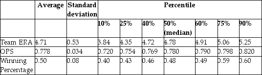  Your regression output is:
$$\begin{array} { l } 
\widehat { \text { Winpct } } = - 0.19 - 0.099 \times \text { teamera } + 1.490 \times \text { ops, } R 2 = 0.92 , \text { SER } = 0.02 \text {. } \
\quad\quad\quad\quad\quad\text { (0.08) (0.008) }\quad\quad\quad\quad\quad\quad(0.126) \
\end{array}$$
(a)Interpret the regression. Are the results statistically significant and important?
(b)There are two leagues in MLB, the American League (AL)and the National League (NL). One major difference is that the pitcher in the AL does not have to bat. Instead there is a "designated hitter" in the hitting line-up. You are concerned that, as a result, there is a different effect of pitching and hitting in the AL from the NL. To test this hypothesis, you allow the AL regression to have a different intercept and different slopes from the NL regression. You therefore create a binary variable for the American League (DAL)and estimate the following specification: $\begin{aligned}
\widehat { \text { Winpct } = - } & 0.29 + 0.10 \times D A L - 0.100 \times \text { teamera } + 0.008 \times ( \text { DAL } \times \text { teamera } ) \
& ( 0.12 ) ( 0.24 ) \quad\quad\quad\quad ( 0.008 )\quad\quad\quad\quad(0.018) \\
& + 1.622 ^ { * } \text { ops } - 0.187 ^ { * } ( D A L \times \text { ops } ) , R 2 = 0.92 , S E R = 0.02 . \
& ( 0.163 ) \quad\quad\quad\quad ( 0.160 )
\end{aligned}$
What is the regression for winning percentage in the AL and NL? Next, calculate the t-statistics and say something about the statistical significance of the AL variables. Since you have allowed all slopes and the intercept to vary between the two leagues, what would the results imply if all coefficients involving DAL were statistically significant?
(c)You remember that sequentially testing the significance of slope coefficients is not the same as testing for their significance simultaneously. Hence you ask your regression package to calculate the F-statistic that all three coefficients involving the binary variable for the AL are zero. Your regression package gives a value of 0.35. Looking at the critical value from you F-table, can you reject the null hypothesis at the 1% level? Should you worry about the small sample size?

Accepted Answer

(a)Lowering the team ERA by one results

Question 6

Using a spreadsheet program such as Excel, plot the following logistic regression function with a single X, $\hat { Y }$ i = 
  $\frac { 1 } { 1 + e ^ { - \left( \hat\beta _ { 0 } + \hat\beta _ { 1 } X _ { i } \right) } }$ , where $\hat { \beta }$ 0 = - 4.13 and $\hat { \beta }$ 1 = 5.37. Enter values of X in the first column starting from 0 and then incrementing these by 0.1 until you reach 2.0. Then enter the logistic function formula in the next column. Finally produce a scatter plot, connecting the predicted values with a line.

Accepted Answer

@#IMG-DLM&_TB5979_00

Question 7

You have collected data for a cross-section of countries in two time periods, 1960 and 1997, say. Your task is to find the determinants for the Wealth of a Nation (per capita income)and you believe that there are three major determinants: investment in physical capital in both time periods (X1,T and X1,0), investment in human capital or education (X2,T and X2,0), and per capita income in the initial period
(Y0). You run the following regression:
ln(YT)= β0 + β1X1,T + β2X1,0 + β3X2,T + β4X1,0 + ln(Y0)+ uT
One of your peers suggests that instead, you should run the growth rate in per capita income over the two periods on the change in physical and human capital. For those results to be a parsimonious presentation of your initial regression, what three restrictions would have to hold? How would you test for these? The same person also points out to you that the intercept vanishes in equations where the data is differenced. Is that correct?

Accepted Answer

The regression using growth rates is as

Question 8

Pages 283-284 in your textbook contain an analysis of the "Return to Education and the Gender Gap." Column (4)in Table 8.1 displays regression results using the 2009 Current Population Survey. The equation below shows the regression result for the same specification, but using the 2005 Current Population Survey. Interpret the major results. $\begin{array} { l } 
\widehat{\text { In eamings }} = 1.215 + 0.0899 \times \text { educ } - 0.521 \times \text { DFemme } + 0.0180 \times ( \text { DFemme } \times \text { educ } ) \
\text { (0.018) (0.0011) } \text { (0.022) } ( 0.0016 ) \\
+ 0.0232 \times \text { exper } - 0.000368 \times \text { exper } 2 - 0.058 \times \text { Midwest } - 0.0098 \times \text { South } - 0.030 \times \text { West } \
( 0.0008 ) \quad \quad\quad \quad\text { (0.000018) \quad \quad\quad \quad\quad \quad} \text { (0.006) } \quad \quad\quad \quad\text { (0.0078) } \quad \quad\quad \quad( 0.0030 ) \
\end{array}$

Accepted Answer

The return to education for males is app

Question 9

The best way to interpret polynomial regressions is to

Accepted Answer

A) take a derivative of Y with respect to the relevant X. 
B) plot the estimated regression function and to calculate the estimated effect on Y associated with a change in X for one or more values of X. 
C) look at the t-statistics for the relevant coefficients. 
D) analyze the standard error of estimated effect. 
A) take a derivative of Y with respect to the relevant X. 
B) plot the estimated regression function and to calculate the estimated effect on Y associated with a change in X for one or more values of X. 
C) look at the t-statistics for the relevant coefficients. 
D) analyze the standard error of estimated effect.

Question 10

You have learned that earnings functions are one of the most investigated relationships in economics. These typically relate the logarithm of earnings to a series of explanatory variables such as education, work experience, gender, race, etc.
(a)Why do you think that researchers have preferred a log-linear specification over a linear specification? In addition to the interpretation of the slope coefficients, also think about the distribution of the error term.
(b)To establish age-earnings profiles, you regress ln(Earn)on Age, where Earn is weekly earnings in dollars, and Age is in years. Plotting the residuals of the regression against age for 1,744 individuals looks as shown in the figure: 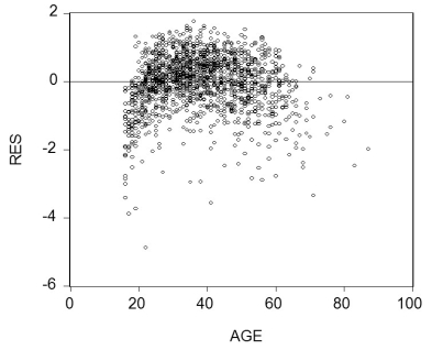  Do you sense a problem?
(c)You decide, given your knowledge of age-earning profiles, to allow the regression line to differ for the below and above 40 years age category. Accordingly you create a binary variable, Dage, that takes the value one for age 39 and below, and is zero otherwise. Estimating the earnings equation results in the following output (using heteroskedasticity-robust standard errors): $\begin{array} { l } 
\widehat { \text { LnEarn } = } 6.92 - 3.13 \times \text { Dage } - 0.019 \times \text { Age } + 0.085 \times ( \text { Dage } \times \text { Age } ) , R 2 = 0.20 , \text { SER } = 0.721 . \
\quad\quad\quad\quad( 38.33 ) ( 0.22 )\quad\quad\quad\quad(0.004)\quad\quad\quad\quad(0.005) \
\end{array}$
Sketch both regression lines: one for the age category 39 years and under, and one for 40 and above. Does it make sense to have a negative sign on the Age coefficient? Predict the ln(earnings)for a 30 year old and a 50 year old. What is the percentage difference between these two?
(d)The F-statistic for the hypothesis that both slopes and intercepts are the same is 124.43. Can you reject the null hypothesis?
(e)What other functional forms should you consider?

Accepted Answer

(a)The error variance and the variance o

Question 11

In nonlinear models, the expected change in the dependent variable for a change in one of the explanatory variables is given by

Accepted Answer

A) △Y = f(X1 + X1, X2,... Xk). 
B) △Y = f(X1 + △X1, X2 + △X2,..., Xk+ △Xk)- f(X1, X2,...Xk). 
C) △Y = f(X1 + △X1, X2,..., Xk)- f(X1, X2,...Xk). 
D) △Y = f(X1 + X1, X2,..., Xk)- f(X1, X2,...Xk). 
A) △Y = f(X1 + X1, X2,... Xk). 
B) △Y = f(X1 + △X1, X2 + △X2,..., Xk+ △Xk)- f(X1, X2,...Xk). 
C) △Y = f(X1 + △X1, X2,..., Xk)- f(X1, X2,...Xk). 
D) △Y = f(X1 + X1, X2,..., Xk)- f(X1, X2,...Xk).

Question 12

Consider the population regression of log earnings [Yi, where Yi = ln(Earningsi)] against two binary variables: whether a worker is married (D1i, where D1i=1 if the ith person is married)and the worker's gender (D2i, where D2i=1 if the ith person is female), and the product of the two binary variables Yi = β0 + β1D1i + β2D2i + β3(D1i×D2i)+ ui. The interaction term

Accepted Answer

A) allows the population effect on log earnings of being married to depend on gender 
B) does not make sense since it could be zero for married males 
C) indicates the effect of being married on log earnings 
D) cannot be estimated without the presence of a continuous variable 
A) allows the population effect on log earnings of being married to depend on gender 
B) does not make sense since it could be zero for married males 
C) indicates the effect of being married on log earnings 
D) cannot be estimated without the presence of a continuous variable

Question 13

To investigate whether or not there is discrimination against a sub-group of individuals, you regress the log of earnings on determining variables, such as education, work experience, etc., and a binary variable which takes on the value of one for individuals in that sub-group and is zero otherwise. You consider two possible specifications. First you run two separate regressions, one for the observations that include the sub-group and one for the others. Second, you run a single regression, but allow for a binary variable to appear in the regression. Your professor suggests that the second equation is better for the task at hand, as long as you allow for a shift in both the intercept and the slopes. Explain her reasoning.

Accepted Answer

By running the regression over the entir

Question 14

Show that for the following regression model
Yt = ${ } _ { e } \beta _ { 0 } + \beta _ { 1 \times t + u }$ where t is a time trend, which takes on the values 1, 2, …,T, β1 represents the instantaneous ("continuous compounding")growth rate. Show how this rate is related to the proportionate rate of growth, which is calculated from the relationship
Yt = Y0 × (1 + g)t
when time is measured in discrete intervals.

Accepted Answer

ln(Y_t)= β₀ + β₁× t + u and hence β₁= @#IMG-DLM&_TB5979

Question 15

Females, it is said, make 70 cents to the dollar in the United States. To investigate this phenomenon, you collect data on weekly earnings from 1,744 individuals, 850 females and 894 males. Next, you calculate their average weekly earnings and find that the females in your sample earned $346.98, while the males made $517.70.
(a)Calculate the female earnings in percent of the male earnings. How would you test whether or not this difference is statistically significant? Give two approaches.
(b)A peer suggests that this is consistent with the idea that there is discrimination against females in the labor market. What is your response?
(c)You recall from your textbook that additional years of experience are supposed to result in higher earnings. You reason that this is because experience is related to "on the job training." One frequently used measure for (potential)experience is "Age-Education-6." Explain the underlying rationale. Assuming, heroically, that education is constant across the 1,744 individuals, you consider regressing earnings on age and a binary variable for gender. You estimate two specifications initially: $\begin{array} { l } 
\widehat { \text { Eam } } = 323.70 + 5.15 \times \text { Age } - 169.78 \times \text { Female } , R 2 = 0.13 , S E R = 274.75 \
\quad\quad\quad\quad (21.18) (0.55)  \quad\quad\quad\quad (13.06) \\
\widehat { \operatorname { Ln } ( \text { Earn } ) } = 5.44 + 0.015 \times \text { Age } - 0.421 \times \text { Female, } R ^ { 2 } = 0.17 , \text { SER } = 0.75 \
\begin{array} { l | l } 
\quad\quad\quad\quad\quad\quad( 0.08 ) ( 0.002 ) &\quad\quad\quad\quad\quad ( 0.036 )
\end{array} \
\end{array}$
where Earn are weekly earnings in dollars, Age is measured in years, and Female is a binary variable, which takes on the value of one if the individual is a female and is zero otherwise. Interpret each regression carefully. For a given age, how much less do females earn on average? Should you choose the second specification on grounds of the higher regression R2?
(d)Your peer points out to you that age-earning profiles typically take on an inverted U-shape. To test this idea, you add the square of age to your log-linear regression. $$\begin{aligned}
\widehat { \operatorname { Ln } ( \text { Earn } ) = } & 3.04 + 0.147 \times \text { Age } - 0.421 \times \text { Female } - 0.0016 \mathrm { Age } ^ { 2 } , \
& ( 0.18 ) ( 0.009 )\quad\quad\quad\quad(0.033)\quad\quad\quad\quad\quad\quad(0.0001)
\end{aligned}$$

$$R ^ { 2 } = 0.28 , S E R = 0.68$$
Interpret the results again. Are there strong reasons to assume that this specification is superior to the previous one? Why is the increase of the Age coefficient so large relative to its value in (c)?
(e)What other factors may play a role in earnings determination?

Accepted Answer

(a)Female earnings are at 67 percent of

Question 16

Indicate whether or not you can linearize the regression functions below so that OLS estimation methods can be applied:
(a)Yi = ${ } _ { e } \beta _ { 0 } + \beta _ { 1 } X _ { i } + u _ { i }$ (b)Yi = $\beta _ { 1 }$ $X _ { 1 i } ^ { \beta _ { 1 } }$ $X _ { 2 i } ^ { \beta _ { 2 } }$ + ui

Accepted Answer

(a)The function can be lineari

Question 17

The binary variable interaction regression

Accepted Answer

A) can only be applied when there are two binary variables, but not three or more. 
B) is the same as testing for differences in means. 
C) cannot be used with logarithmic regression functions because ln(0)is not defined. 
D) allows the effect of changing one of the binary independent variables to depend on the value of the other binary variable. 
A) can only be applied when there are two binary variables, but not three or more. 
B) is the same as testing for differences in means. 
C) cannot be used with logarithmic regression functions because ln(0)is not defined. 
D) allows the effect of changing one of the binary independent variables to depend on the value of the other binary variable.

Question 18

The following are properties of the logarithm function with the exception of

Accepted Answer

A) ln(1/ x)= -ln(x). 
B) ln(a + x)= ln(a)+ ln(x). 
C) ln(ax)= ln(a)+ ln(x). 
D) ln(xa)a ln(x). 
A) ln(1/ x)= -ln(x). 
B) ln(a + x)= ln(a)+ ln(x). 
C) ln(ax)= ln(a)+ ln(x). 
D) ln(xa)a ln(x).

Question 19

Consider a typical beta convergence regression function from macroeconomics, where the growth of a country's per capita income is regressed on the initial level of per capita income and various other economic and socio-economic variables. Assume that two of these variables are the average number of years of education in the specific country and a binary variable which indicates whether or not the country experienced a significant number of years of civil war/unrest. Explain why it would make sense to have these two variables enter separately and also why you should use an interaction term. What signs would you expect on the three coefficients?

Accepted Answer

Simple extensions of the standard neocla

Question 20

You have been asked by your younger sister to help her with a science fair project. During the previous years she already studied why objects float and there also was the inevitable volcano project. Having learned regression techniques recently, you suggest that she investigate the weight-height relationship of 4th to 6th graders. Her presentation topic will be to explain how people at carnivals predict weight. You collect data for roughly 100 boys and girls between the ages of nine and twelve and estimate for her the following relationship: 
$\begin{array} { c } 
\widehat { \text { Weight } } = 45.59 + 4.32 \times \text { Height } ^ { 4 } , R ^ { 2 } = 0.55 , \text { SER } = 15.69 \
( 3.81 ) \quad ( 0.46 )
\end{array}$
where Weight is in pounds, and Height4 is inches above 4 feet.
(a)Interpret the results.
(b)You remember from the medical literature that females in the adult population are, on average, shorter than males and weigh less. You also seem to have heard that females, controlling for height, are supposed to weigh less than males. To see if this relationship holds for children, you add a binary variable (DFY)that takes on the value one for girls and is zero otherwise. You estimate the following regression function: $\begin{array} { l } 
\widehat { \text { Weight } } = 36.27 + 17.33 \times \text { DFY } + 5.32 \times \text { Height } 4 - 1.83 \times ( \text { DFY } \times \text { Height } 4 ) \
\quad\quad\quad\quad( 5.99 ) \quad ( 7.36 ) \quad\quad\quad(0.80)\quad\quad\quad\quad(0.90)\
\end{array}$

$$R ^ { 2 } =0.58 , S E R = 15.41$$
Are the signs on the new coefficients as expected? Are the new coefficients individually statistically significant? Write down and sketch the regression function for boys and girls separately.
(c)The medical literature provides you with the following information for median height and weight of nine- to twelve-year-olds:
Median Height and Weight for Children, Age 9-12 $$\begin{array} { | l | c | c | c | c | } 
\hline & \text { Boys' Weight } & \text { Boys' Height } & \text { Girls' Weight } & \text { Girls' Height } \
\hline \text { 9-year-old } & 60 & 52 & 60 & 49 \
\hline \text { 10-year-old } & 70 & 54 & 70 & 52 \
\hline \text { 11-year-old } & 77 & 56 & 80 & 57 \
\hline \text { 12-year-old } & 87 & 58.5 & 92 & 60 \
\hline
\end{array}$$ Insert two height/weight measures each for boys and girls and see how accurate your predictions are.
(d)The F-statistic for testing that the intercept and slope for boys and girls are identical is 2.92. Find the critical values at the 5% and 1% level, and make a decision. Allowing for a different intercept with an identical slope results in a t-statistic for DFY of (-0.35). Having identical intercepts but different slopes gives a t-statistic on (DFYHeight4)of (-0.35)also. Does this affect your previous conclusion?
(e)Assume that you also wanted to test if the relationship changes by age. Briefly outline how you would specify the regression including the gender binary variable and an age binary variable (Older)that takes on a value of one for eleven to twelve year olds and is zero otherwise. Indicate in a table of two rows and two columns how the estimated relationship would vary between younger girls, older girls, younger boys, and older boys.

Accepted Answer

(a)For every inch above 4 feet, children

Including an interaction term between two independent variables, X₁ and X₂, allows for the following except:

(Requires Calculus)Show that for the log-log model the slope coefficient is the elasticity.

Sketch for the log-log model what the relationship between Y and X looks like for various parameter values of the slope, i.e., β₁ > 1; 0 < β₁ < 1; β₁= (-1).

The best way to interpret polynomial regressions is to

In nonlinear models, the expected change in the dependent variable for a change in one of the explanatory variables is given by

Indicate whether or not you can linearize the regression functions below so that OLS estimation methods can be applied: (a)Y_i = ${ } _ { e } \beta _ { 0 } + \beta _ { 1 } X _ { i } + u _ { i }$ (b)Y_i = $\beta _ { 1 }$ $X _ { 1 i } ^ { \beta _ { 1 } }$ $X _ { 2 i } ^ { \beta _ { 2 } }$ + u_i

The binary variable interaction regression

The following are properties of the logarithm function with the exception of

Economic Questions and Data

Review of Probability

Review of Statistics

Linear Regression With One Regressor

Regression With a Single Regressor: Hypothesis Tests and Confidence Intervals

Linear Regression With Multiple Regressors

Hypothesis Tests and Confidence Intervals in Multiple Regression

Assessing Studies Based on Multiple Regression

Regression With Panel Data

Regression With a Binary Dependent Variable

Instrumental Variables Regression

Experiments and Quasi-Experiments

Introduction to Time Series Regression and Forecasting

Estimation of Dynamic Causal Effects

Additional Topics in Time Series Regression

The Theory of Linear Regression With One Regressor

The Theory of Multiple Regression

Filters

Exam 8: Nonlinear Regression Functions

Including an interaction term between two independent variables, X1 and X2, allows for the following except:

(Requires Calculus)Show that for the log-log model the slope coefficient is the elasticity.

Sketch for the log-log model what the relationship between Y and X looks like for various parameter values of the slope, i.e., β1 > 1; 0 < β1 < 1; β1 = (-1).

The best way to interpret polynomial regressions is to

In nonlinear models, the expected change in the dependent variable for a change in one of the explanatory variables is given by

The binary variable interaction regression

The following are properties of the logarithm function with the exception of

Economic Questions and Data

Review of Probability

Review of Statistics

Linear Regression With One Regressor

Regression With a Single Regressor: Hypothesis Tests and Confidence Intervals

Linear Regression With Multiple Regressors

Hypothesis Tests and Confidence Intervals in Multiple Regression

Assessing Studies Based on Multiple Regression

Regression With Panel Data

Regression With a Binary Dependent Variable

Instrumental Variables Regression

Experiments and Quasi-Experiments

Introduction to Time Series Regression and Forecasting

Estimation of Dynamic Causal Effects

Additional Topics in Time Series Regression

The Theory of Linear Regression With One Regressor

The Theory of Multiple Regression

Filters

Including an interaction term between two independent variables, X₁ and X₂, allows for the following except:

Sketch for the log-log model what the relationship between Y and X looks like for various parameter values of the slope, i.e., β₁ > 1; 0 < β₁ < 1; β₁= (-1).