Exam 7: Hypothesis Tests and Confidence Intervals in Multiple Regression
Exam 1: Economic Questions and Data17 Questions
Exam 2: Review of Probability70 Questions
Exam 3: Review of Statistics65 Questions
Exam 4: Linear Regression With One Regressor65 Questions
Exam 5: Regression With a Single Regressor: Hypothesis Tests and Confidence Intervals59 Questions
Exam 6: Linear Regression With Multiple Regressors65 Questions
Exam 7: Hypothesis Tests and Confidence Intervals in Multiple Regression64 Questions
Exam 8: Nonlinear Regression Functions63 Questions
Exam 9: Assessing Studies Based on Multiple Regression65 Questions
Exam 10: Regression With Panel Data50 Questions
Exam 11: Regression With a Binary Dependent Variable50 Questions
Exam 12: Instrumental Variables Regression50 Questions
Exam 13: Experiments and Quasi-Experiments50 Questions
Exam 14: Introduction to Time Series Regression and Forecasting50 Questions
Exam 15: Estimation of Dynamic Causal Effects50 Questions
Exam 16: Additional Topics in Time Series Regression50 Questions
Exam 17: The Theory of Linear Regression With One Regressor49 Questions
Exam 18: The Theory of Multiple Regression50 Questions
Select questions type
The homoskedasticity-only F-statistic is given by the following formula
Free
(Multiple Choice)
4.9/5  (36)
(36)
Correct Answer: Verified
A
A 95% confidence set for two or more coefficients is a set that contains
Free
(Multiple Choice)
4.8/5 (32)
Correct Answer:Verified
D
If the absolute value of your calculated t-statistic exceeds the critical value from the standard normal distribution you can
Free
(Multiple Choice)
4.8/5 (33)
Correct Answer:Verified
B
In the multiple regression model with two explanatory variables
Yi = ?0 + ?1X1i + ?2X2i + ui
the OLS estimators for the three parameters are as follows (small letters refer to deviations from means as in zi = Zi - ): You have collected data for 104 countries of the world from the Penn World Tables and want to estimate the effect of the population growth rate (X1i)and the saving rate (X2i)(average investment share of GDP from 1980 to 1990)on GDP per worker (relative to the U.S.)in 1990. The various sums needed to calculate the OLS estimates are given below: = 33.33; = 2.025; =17.313 = 8.3103; = .0122; = 0.6422 = - 0.2304; = 1.5676; = -0.0520
The heteroskedasticity-robust standard errors of the two slope coefficients are 1.99 (for population growth)and 0.23 (for the saving rate). Calculate the 95% confidence interval for both coefficients. How many standard deviations are the coefficients away from zero?
(Essay)
4.8/5 (34)
Consider the following regression output for an unrestricted and a restricted model.
Unrestricted model:
Dependent Variable: TESTSCR
Method: Least Squares
Date: 07/31/06 Time: 17:35
Sample: 1 420
Included observations: 420 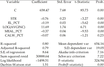 Restricted model:
Dependent Variable: TESTSCR
Method: Least Squares
Date: 07/31/06 Time: 17:37
Sample: 1 420
Included observations: 420
Restricted model:
Dependent Variable: TESTSCR
Method: Least Squares
Date: 07/31/06 Time: 17:37
Sample: 1 420
Included observations: 420 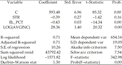 Calculate the homoskedasticity only F-statistic and determine whether the null hypothesis can be rejected at the 5% significance level.
(Essay)
4.7/5 (36)
Attendance at sports events depends on various factors. Teams typically do not change ticket prices from game to game to attract more spectators to less attractive games. However, there are other marketing tools used, such as fireworks, free hats, etc., for this purpose. You work as a consultant for a sports team, the Los Angeles Dodgers, to help them forecast attendance, so that they can potentially devise strategies for price discrimination. After collecting data over two years for every one of the 162 home games of the 2000 and 2001 season, you run the following regression: = 15,005 + 201 × Temperat + 465 × DodgNetWin + 82 × OppNetWin
(8,770)(121)(169)(26)
+ 9647 × DFSaSu + 1328 × Drain + 1609 × D150m + 271 × DDiv - 978 × D2001;
(1505)(3355)(1819)(1,184)(1,143)
R2=0.416, SER = 6983
where Attend is announced stadium attendance, Temperat it the average temperature on game day, DodgNetWin are the net wins of the Dodgers before the game (wins-losses), OppNetWin is the opposing team's net wins at the end of the previous season, and DFSaSu, Drain, D150m, Ddiv, and D2001 are binary variables, taking a value of 1 if the game was played on a weekend, it rained during that day, the opposing team was within a 150 mile radius, the opposing team plays in the same division as the Dodgers, and the game was played during 2001, respectively. Numbers in parentheses are heteroskedasticity- robust standard errors.
(a)Are the slope coefficients statistically significant?
(b)To test whether the effect of the last four binary variables is significant, you have your regression program calculate the relevant F-statistic, which is 0.295. What is the critical value? What is your decision about excluding these variables?
(Essay)
4.8/5 (36)
The overall regression F-statistic tests the null hypothesis that
(Multiple Choice)
4.9/5 (44)
Consider the following Cobb-Douglas production function Yi = AK i L i (where Y is output, A is the level of technology, K is the capital stock, and L is the labor force), which has been linearized here (by using logarithms)to look as follows:
yi = + β1ki + β2li + ui
Assuming that the errors are heteroskedastic, you want to test for constant returns to scale. Using a t-statistic and "Approach #2," how would you proceed.
(Essay)
4.9/5 (41)
You have estimated the following regression to explain hourly wages, using a sample of 250 individuals: = -2.44 - 1.57 × DFemme + 0.27 × DMarried + 0.59 × Educ + 0.04 × Exper - 0.60 × DNonwhite
(1.29)(0.33)(0.36)(0.09)(0.01)(0.49)
+ 0.13 × NCentral - 0.11 × South
(0.59)(0.58)
R2 = 0.36, SER = 2.74, n = 250
Test the null hypothesis that the coefficients on DMarried, DNonwhite, and the two regional variables, NCentral and South are zero. The F-statistic for the null hypothesis βmarried = βnonwhite = βnonwhite = βncentral = βsouth = 0 is 0.61. Do you reject the null hypothesis?
(Essay)
4.8/5 (37)
Consider the regression model Yi = ?0 + ?1X1i + ?2X2i+ ?3X3i + ui. Use "Approach #2" from Section 7.3 to transform the regression so that you can use a t-statistic to test:
?1 =
(Essay)
4.8/5 (29)
Give an intuitive explanation for 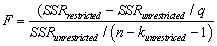 Name conditions under which the F-statistic is large and hence rejects the null hypothesis.
(Essay)
4.8/5 (30)
If you reject a joint null hypothesis using the F-test in a multiple hypothesis setting, then
(Multiple Choice)
4.9/5 (31)
When testing the null hypothesis that two regression slopes are zero simultaneously, then you cannot reject the null hypothesis at the 5% level, if the ellipse contains the point
(Multiple Choice)
4.9/5 (39)
The general answer to the question of choosing the scale of the variables is
(Multiple Choice)
4.8/5 (29)
When your multiple regression function includes a single omitted variable regressor, then
(Multiple Choice)
5.0/5 (39)
The F-statistic with q = 2 restrictions when testing for the restrictions ?1 = 0 and ?2 = 0 is given by the following formula: Discuss how this formula can be understood intuitively.
(Essay)
4.9/5 (33)
In the multiple regression model, the t-statistic for testing that the slope is significantly different from zero is calculated
(Multiple Choice)
4.7/5 (38)
The cost of attending your college has once again gone up. Although you have been told that education is investment in human capital, which carries a return of roughly 10% a year, you (and your parents)are not pleased. One of the administrators at your university/college does not make the situation better by telling you that you pay more because the reputation of your institution is better than that of others. To investigate this hypothesis, you collect data randomly for 100 national universities and liberal arts colleges from the 2000-2001 U.S. News and World Report annual rankings. Next you perform the following regression = 7,311.17 + 3,985.20 × Reputation - 0.20 × Size
(2,058.63)(664.58)(0.13)
+ 8,406.79 × Dpriv - 416.38 × Dlibart - 2,376.51 × Dreligion
(2,154.85)(1,121.92)(1,007.86)
R2=0.72, SER = 3,773.35
where Cost is Tuition, Fees, Room and Board in dollars, Reputation is the index used in U.S. News and World Report (based on a survey of university presidents and chief academic officers), which ranges from 1 ("marginal")to 5 ("distinguished"), Size is the number of undergraduate students, and Dpriv, Dlibart, and Dreligion are binary variables indicating whether the institution is private, a liberal arts college, and has a religious affiliation. The numbers in parentheses are heteroskedasticity-robust standard errors.
(a)Indicate whether or not the coefficients are significantly different from zero.
(b)What is the p-value for the null hypothesis that the coefficient on Size is equal to zero? Based on this, should you eliminate the variable from the regression? Why or why not?
(c)You want to test simultaneously the hypotheses that βsize = 0 and βDilbert = 0. Your regression package returns the F-statistic of 1.23. Can you reject the null hypothesis?
(d)Eliminating the Size and Dlibart variables from your regression, the estimation regression becomes = 5,450.35 + 3,538.84 × Reputation + 10,935.70 × Dpriv - 2,783.31 × Dreligion;
(1,772.35)(590.49)(875.51)(1,180.57)
R2=0.72, SER = 3,792.68
Why do you think that the effect of attending a private institution has increased now?
(e)You give a final attempt to bring the effect of Size back into the equation by forcing the assumption of homoskedasticity onto your estimation. The results are as follows: = 7,311.17 + 3,985.20 × Reputation - 0.20 × Size
(1,985.17)(593.65)(0.07)
+ 8,406.79 × Dpriv - 416.38 × Dlibart - 2,376.51 × Dreligion
(1,423.59)(1,096.49)(989.23)
R2=0.72, SER = 3,682.02
Calculate the t-statistic on the Size coefficient and perform the hypothesis test that its coefficient is zero. Is this test reliable? Explain.
(Essay)
4.8/5 (33)
Consider a situation where economic theory suggests that you impose certain restrictions on your estimated multiple regression function. These may involve the equality of parameters, such as the returns to education and on the job training in earnings functions, or the sum of coefficients, such as constant returns to scale in a production function. To test the validity of your restrictions, you have your statistical package calculate the corresponding F-statistic. Find the critical value from the F-distribution at the 5% and 1% level, and comment whether or not you will reject the null hypothesis in each of the following cases.
(a)number of observations: 152; number of restrictions: 3; F-statistic: 3.21
(b)number of observations: 1,732; number of restrictions:7; F-statistic: 4.92
(c)number of observations: 63; number of restrictions: 1; F-statistic: 2.47
(d)number of observations: 4,000; number of restrictions: 5; F-statistic: 1.82
(e)Explain why you can use the Fq,∞ distribution to compute the critical values in (a)-(d).
(Essay)
4.9/5 (29)
Filters
- Essay(0)
- Multiple Choice(0)
- Short Answer(0)
- True False(0)
- Matching(0)