Exam 9: Forecasting
Heidi favors using a two period moving average but Tim is "an exponential-smoothing man." Tim's demand forecast for May was identical to Heidi's. What value of alpha would Tim need to use in order for his June forecast to be identical to Heidi's if each sticks with their preferred technique? Note that Tim's forecast for May was identical to Heidi's two-period moving average for May. Month Demand January 154 February 148 March 214 April 180 May 225 June 246
B
Which of these quantitative techniques can be a causal model?
A
Using the data in the table, first plot the data and comment on the appearance of the demand pattern. Then develop a forecast for periods 51-70 that fits the data.
Time Output Time Output Time Output Time Output 1 12.5 14 16.4 27 -19.2 40 11.3 2 14.8 15 11.7 28 10.6 41 11.1 3 15.3 16 11.1 29 16.8 42 52.5 4 15 17 11.9 30 22.5 43 11.3 5 11.5 18 11.3 31 15.5 44 -19.3 6 11.6 19 13.7 32 11.7 45 12 7 12.8 20 16.3 33 11.9 46 15.5 8 51.9 21 13.1 34 13 47 20.5 9 11 22 10.8 35 11.9 48 16.5 10 -19.7 23 10.3 36 13.5 49 12.5 11 11.9 24 11 37 16.5 50 10.5 12 17.8 25 51.4 38 14 13 20.3 26 11.6 39 11
Data are highly seasonal as the graph and data table indicate. 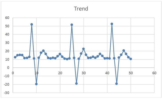 Peaks near 50 occur at points 8, 25 and 42, and this seasonality is reflected in the other significant features of the graph, e.g., lows near -20 at points 10, 27 and 44. The data are rearranged in this table into three 17 observation rows (since 17 is the period of this function)with a seasonal average and seasonal relative appended to the right. The overall average for the data is 13.828; the column labeled "Seasonal" is each average divided by the 13.828 figure.
Divide each entry in the table by the seasonal relative. Then use linear regression with independent variables ranging from 1-50 to yield the regression equation
Output = 14.05629-0.00895 ∗ Time
Reseasoning the forecasted values by the seasonal relatives gives the results in the table and the graph below.
The graph below is a plot of the original data for points 1-50 and the forecast points 51-70. 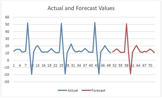
"A simple moving average was good enough for my dad, and it's good enough for me," Ethan declared as he prepared his forecast. The assistant dean knew that the size of incoming MBA classes had been increasing dramatically over the previous few semesters and that the forecasts Ethan would prepare using his father's method would ________ the actual size of the incoming class.
What are the laws of forecasting and what are their implications for operations and supply chain managers?
Heidi runs a multiple regression for the output of cheese curds by using the daily temperature and the consumption of sweet clover. The intercept term is 23, the slope coefficient for the daily temperature is 1.5 and the slope coefficient for the consumption of sweet clover is 0; both coefficients are statistically significant. Which of these conclusions is most appropriate?
The Pancake House did a brisk business on the weekend and the maître d' was always on the lookout for ways to improve the customer experience. He carefully tracked the number of customers that graced their establishment over the last four weekends. He was hopeful that he could forecast the number of customers that would come for the world's finest pancakes the next weekend.
Weekend 1 Weekend 2 Weekend 3 Weekend 4 Friday 131 216 286 355 Saturday 225 311 408 490 Sunday 166 249 330 415 Using the data in the table, first plot the data and comment on the appearance of the demand pattern. Then develop a forecast for weekend #5 that fits the data.
A poultry farmer that dabbles in statistics is interested in exploring the relationship between two types of feed (layer pellets and scratch), water, and the output of his laying hens. For ten days he records the number of ounces of layer pellets and scratch the hens consume and the number of fluid ounces of water and tracks the number of eggs that are produced. What is his regression equation based on the data?
Scratch Layer Pellets Water Eggs 48 29 36 24 44 27 34 22 41 22 31 20 42 21 32 20 48 23 34 22 44 28 34 23 42 22 37 21 41 28 33 22 42 22 31 20 47 29 37 24
As yet another earthquake rattled his china cabinet, the data scientist vowed to once and for all determine whether hydraulic fracturing (where water is injected into the earth)was predictive of the number of earthquakes in the region. Using the data below, what evidence can you find to support the notion that the number of injections helps explain the number of earthquakes in the region?
Injections Earthquakes 137 682 331 833 360 905 442 1008 478 1482 529 1742
The greater the randomness in the data, the ________ the value of the alpha should be in an exponential smoothing forecast.
The tracking signal calculated for the first forecast is always either +1 or -1.
A firm's demand data from the last two quarters is displayed in the table. Use a three period moving average to forecast demand for July. Month Demand January 154 February 148 March 214 April 180 May 225 June 246
The independent variable is the quantity the forecaster is interested in estimating with a linear regression model.
The forecast data matches the actual data perfectly if the mean absolute deviation is 0.0.
A forecaster is assessing two different models for demand. The output from each model and the actual demand data appear in the table. Use MAD and a tracking signal to compare the two models. Which model does a better job of forecasting?
Demand Model 1 Model 2 52 55.0 51.0 52 54.7 51.9 60 54.4 52.0 56 55.0 59.2 58 55.1 56.3 58 55.4 57.8 52 55.6 58.0 57 55.3 52.6 53 55.4 56.6 57 55.2 53.4
Models that predict values based upon some independent factor(s)other than time are ________ forecasting models.
A seasonal pattern in time series data is evident when the level of the variable of interest moves erratically up or down from one period to the next.
McMahon and Tate advertising company is interested in an appropriate mix of print, radio, and television ads for their new client. Darrin Stevens performs a multiple regression on the effects of dollars spent on each type of media on dollars of sales of product. Darrin uses data from the most recent advertising campaigns and develops the following equation: y = 254,215 + 6.79 × Print - 1.4 × Radio + 16.87 × Television
The r-squared statistic is 0.77 and all coefficients are significant. Which of the following statements is best?
Fed up with her working conditions at the call center, Lisa decides to invest in a state-of-the-art sewing machine and produce limited quantities of her own clothing designs. After a few months of operation, she decides to apply some of the forecasting techniques she mastered in school. Which of these statements about her forecasts is correct?
Qualitative forecasts are used when there is plenty of relevant data.
Filters
- Essay(0)
- Multiple Choice(0)
- Short Answer(0)
- True False(0)
- Matching(0)