Exam 17: A Roadmap for Analyzing Data
Exam 1: Defining and Collecting Data189 Questions
Exam 3: Numerical Descriptive Measures184 Questions
Exam 4: Basic Probability156 Questions
Exam 5: Discrete Probability Distributions218 Questions
Exam 6: The Normal Distribution and Other Continuous Distributions189 Questions
Exam 7: Sampling Distributions127 Questions
Exam 8: Confidence Interval Estimation196 Questions
Exam 9: Fundamentals of Hypothesis Testing: One-Sample Tests170 Questions
Exam 10: Two-Sample Tests210 Questions
Exam 11: Analysis of Variance130 Questions
Exam 12: Chi-Square Tests and Nonparametric Tests175 Questions
Exam 13: Simple Linear Regression213 Questions
Exam 14: Introduction to Multiple Regression337 Questions
Exam 15: Multiple Regression Model Building96 Questions
Exam 16: Time-Series Forecasting165 Questions
Exam 17: A Roadmap for Analyzing Data303 Questions
Exam 18: Statistical Applications in Quality Management130 Questions
Exam 19: Decision Making126 Questions
Exam 20: Index Numbers44 Questions
Exam 21: Chi-Square Tests for the Variance or Standard Deviation11 Questions
Exam 22: Mcnemar Test for the Difference Between Two Proportions Related Samples15 Questions
Exam 25: The Analysis of Means Anom2 Questions
Exam 23: The Analysis of Proportions Anop3 Questions
Exam 24: The Randomized Block Design85 Questions
Exam 26: The Power of a Test41 Questions
Exam 27: Estimation and Sample Size Determination for Finite Populations13 Questions
Exam 28: Application of Confidence Interval Estimation in Auditing13 Questions
Exam 29: Sampling From Finite Populations20 Questions
Exam 30: The Normal Approximation to the Binomial Distribution27 Questions
Exam 31: Counting Rules14 Questions
Exam 32: Lets Get Started Big Things to Learn First33 Questions
Select questions type
Data on the amount of money made in a year by 1,000 families in a small town were collected.You want to know how much each family will get if the money made by all the 1,000 families is pooled together and then evenly redistributed back to them.Which of the following would you compute?
(Multiple Choice)
4.7/5  (41)
(41)
True or False: Every spring semester,the School of Business coordinates a luncheon for graduating seniors,their families,and friends with local business leaders .Corporate sponsorship pays for the lunches of each of the seniors,but students have to purchase tickets to cover the cost of lunches served to guests they bring with them.Data on the number of guests each graduating senior invited to the luncheon and the number of graduating seniors in each category were collected.A histogram can be used to present this information.
(True/False)
4.8/5 (37)
Data on the amount of money made in a year by 1,000 families in a small town were collected.You want to know the difference in the amount of money made in that year by the middle 50% of the 1,000 families.Which of the following would you compute?
(Multiple Choice)
4.8/5 (39)
Are Japanese managers more motivated than American managers? A randomly selected group of 100 managers from each group were administered the Sarnoff Survey of Attitudes Toward Life (SSATL),which measures motivation for upward mobility.The mean and standard deviation of the SSATL scores are computed.The standard deviations of the SSATL scores suggest that the standard deviation from the two groups is very different.Which of the following tests will be the most appropriate?
(Multiple Choice)
4.8/5 (32)
TABLE 17-12
The marketing manager for a nationally franchised lawn service company would like to study the characteristics that differentiate home owners who do and do not have a lawn service.A random sample of 30 home owners located in a suburban area near a large city was selected; 15 did not have a lawn service (code 0)and 15 had a lawn service (code 1).Additional information available concerning these 30 home owners includes family income (Income,in thousands of dollars),lawn size (Lawn Size,in thousands of square feet),attitude toward outdoor recreational activities (Attitude 0 = unfavorable,1 = favorable),number of teenagers in the household (Teenager),and age of the head of the household (Age).
The Minitab output is given below: 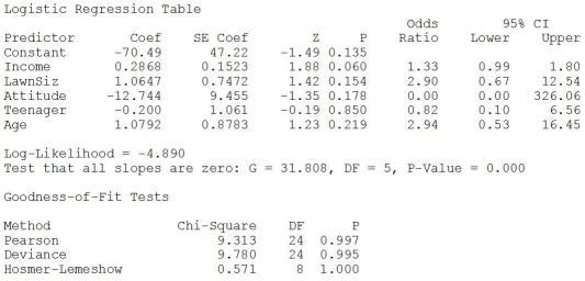 -True or False: Referring to Table 17-12,there is not enough evidence to conclude that Teenager makes a significant contribution to the model in the presence of the other independent variables at a 0.05 level of significance.
(True/False)
4.9/5 (29)
TABLE 17-1
A real estate builder wishes to determine how house size (House)is influenced by family income (Income),family size (Size),and education of the head of household (School).House size is measured in hundreds of square feet,income is measured in thousands of dollars,and education is in years.The builder randomly selected 50 families and ran the multiple regression.Microsoft Excel output is provided below: 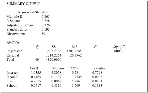 -Referring to Table 17-1,when the builder used a simple linear regression model with house size (House)as the dependent variable and education (School)as the independent variable,he obtained an r2 value of 23.0%.What additional percentage of the total variation in house size has been explained by including family size and income in the multiple regression?
(Multiple Choice)
4.7/5 (37)
TABLE 17-10
Given below are results from the regression analysis where the dependent variable is the number of weeks a worker is unemployed due to a layoff (Unemploy)and the independent variables are the age of the worker (Age),the number of years of education received (Edu),the number of years at the previous job (Job Yr),a dummy variable for marital status (Married: 1 = married,0 = otherwise),a dummy variable for head of household (Head: 1 = yes,0 = no)and a dummy variable for management position (Manager: 1 = yes,0 = no).We shall call this Model 1.The coefficient of partial determination ( 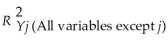 )of each of the 6 predictors are,respectively,0.2807,0.0386,0.0317,0.0141,0.0958,and 0.1201.
 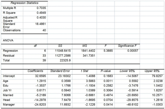 Model 2 is the regression analysis where the dependent variable is Unemploy and the independent variables are Age and Manager.The results of the regression analysis are given below:
 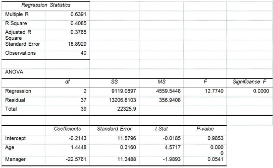 -True or False: Referring to Table 17-10,Model 1,there is sufficient evidence that the number of weeks a worker is unemployed due to a layoff depends on all of the explanatory variables at a 10% level of significance.
(True/False)
4.9/5 (36)
TABLE 17-12
The marketing manager for a nationally franchised lawn service company would like to study the characteristics that differentiate home owners who do and do not have a lawn service.A random sample of 30 home owners located in a suburban area near a large city was selected; 15 did not have a lawn service (code 0)and 15 had a lawn service (code 1).Additional information available concerning these 30 home owners includes family income (Income,in thousands of dollars),lawn size (Lawn Size,in thousands of square feet),attitude toward outdoor recreational activities (Attitude 0 = unfavorable,1 = favorable),number of teenagers in the household (Teenager),and age of the head of the household (Age).
The Minitab output is given below:
-Referring to Table 17-12,what is the p-value of the test statistic when testing whether the model is a good-fitting model?
(Short Answer)
4.8/5 (45)
TABLE 17-2
One of the most common questions of prospective house buyers pertains to the cost of heating in dollars (Y).To provide its customers with information on that matter,a large real estate firm used the following 4 variables to predict heating costs: the daily minimum outside temperature in degrees of Fahrenheit (X1),the amount of insulation in inches (X2),the number of windows in the house (X3),and the age of the furnace in years (X4).Given below are the EXCEL outputs of two regression models. 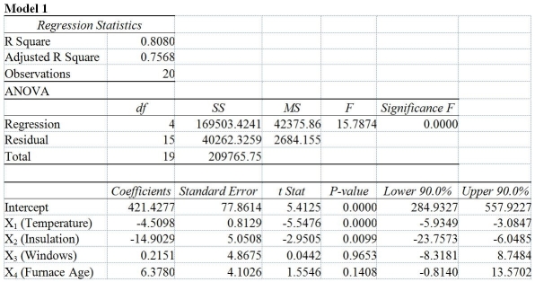
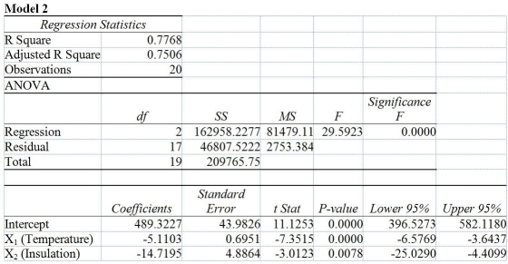 -Referring to Table 17-2,what are the degrees of freedom of the partial F test for H0 : β3 = β4 = 0 vs.H1 : At least one βj ≠ 0,j = 3,4?
(Multiple Choice)
4.7/5 (40)
TABLE 17-8
The superintendent of a school district wanted to predict the percentage of students passing a sixth-grade proficiency test.She obtained the data on percentage of students passing the proficiency test (% Passing),daily mean of the percentage of students attending class (% Attendance),mean teacher salary in dollars (Salaries),and instructional spending per pupil in dollars (Spending)of 47 schools in the state.
Following is the multiple regression output with Y = % Passing as the dependent variable,X1 = % Attendance,X2 = Salaries and X3 = Spending: 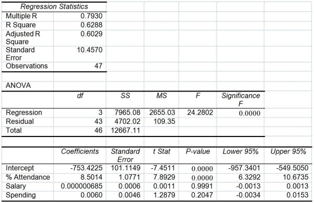 -Referring to Table 17-8,what are the numerator and denominator degrees of freedom,respectively,for the test statistic to determine whether there is a significant relationship between the percentage of students passing the proficiency test and the entire set of explanatory variables?
(Short Answer)
4.7/5 (30)
TABLE 17-12
The marketing manager for a nationally franchised lawn service company would like to study the characteristics that differentiate home owners who do and do not have a lawn service.A random sample of 30 home owners located in a suburban area near a large city was selected; 15 did not have a lawn service (code 0)and 15 had a lawn service (code 1).Additional information available concerning these 30 home owners includes family income (Income,in thousands of dollars),lawn size (Lawn Size,in thousands of square feet),attitude toward outdoor recreational activities (Attitude 0 = unfavorable,1 = favorable),number of teenagers in the household (Teenager),and age of the head of the household (Age).
The Minitab output is given below:
-True or False: Referring to Table 17-12,there is not enough evidence to conclude that the model is not a good-fitting model at a 0.05 level of significance.
(True/False)
4.9/5 (33)
TABLE 17-9
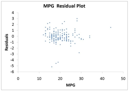
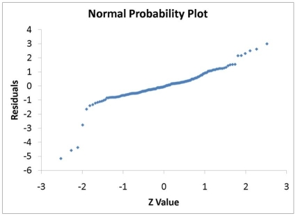
What are the factors that determine the acceleration time (in sec.)from 0 to 60 miles per hour of a car? Data on the following variables for 171 different vehicle models were collected:
Accel Time: Acceleration time in sec.
Cargo Vol: Cargo volume in cu.ft.
HP: Horsepower
MPG: Miles per gallon
SUV: 1 if the vehicle model is an SUV with Coupe as the base when SUV and Sedan are both 0
Sedan: 1 if the vehicle model is a sedan with Coupe as the base when SUV and Sedan are both 0
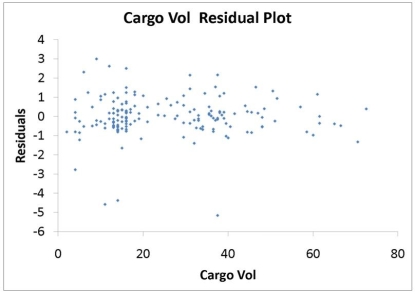
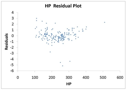
The regression results using acceleration time as the dependent variable and the remaining variables as the independent variables are presented below. 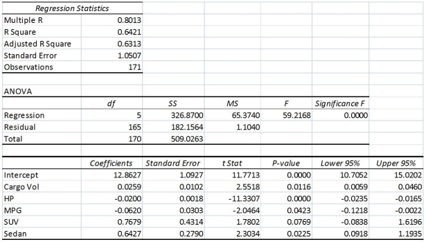 The various residual plots are as shown below.
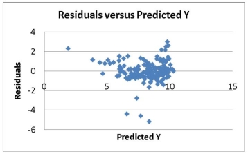
 The coefficient of partial determination (
 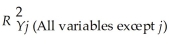 )of each of the 5 predictors are,respectively,0.0380,0.4376,0.0248,0.0188,and 0.0312.
The coefficient of multiple determination for the regression model using each of the 5 variables Xj as the dependent variable and all other X variables as independent variables (
)of each of the 5 predictors are,respectively,0.0380,0.4376,0.0248,0.0188,and 0.0312.
The coefficient of multiple determination for the regression model using each of the 5 variables Xj as the dependent variable and all other X variables as independent variables (  )are,respectively,0.7461,0.5676,0.6764,0.8582,0.6632.
-Referring to Table 17-9,what is the value of the test statistic to determine whether SUV makes a significant contribution to the regression model in the presence of the other independent variables at a 5% level of significance?
)are,respectively,0.7461,0.5676,0.6764,0.8582,0.6632.
-Referring to Table 17-9,what is the value of the test statistic to determine whether SUV makes a significant contribution to the regression model in the presence of the other independent variables at a 5% level of significance?
(Short Answer)
4.8/5 (31)
A certain type of rare gem serves as a status symbol for many of its owners.In theory,for low prices,the demand increases and it decreases as the price of the gem increases.However,experts hypothesize that when the gem is valued at very high prices,the demand increases with price due to the status owners believe they gain in obtaining the gem.Data on price and quantity sold were collected for a sample of 35 rare gems of this type.Which of the following would be the most appropriate analysis to perform?
(Multiple Choice)
4.8/5 (41)
TABLE 17-3
A financial analyst wanted to examine the relationship between salary (in $1,000)and 4 variables: age (X1 = Age),experience in the field (X2 = Exper),number of degrees (X3 = Degrees),and number of previous jobs in the field (X4 = Prevjobs).He took a sample of 20 employees and obtained the following Microsoft Excel output:
SUMMARY OUTPUT
Regression Statistics 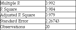 ANOVA
ANOVA 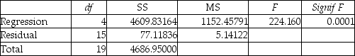
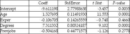 -Referring to Table 17-3,the p-value of the F test for the significance of the entire regression is ________.
(Short Answer)
4.8/5 (26)
TABLE 17-10
Given below are results from the regression analysis where the dependent variable is the number of weeks a worker is unemployed due to a layoff (Unemploy)and the independent variables are the age of the worker (Age),the number of years of education received (Edu),the number of years at the previous job (Job Yr),a dummy variable for marital status (Married: 1 = married,0 = otherwise),a dummy variable for head of household (Head: 1 = yes,0 = no)and a dummy variable for management position (Manager: 1 = yes,0 = no).We shall call this Model 1.The coefficient of partial determination ( )of each of the 6 predictors are,respectively,0.2807,0.0386,0.0317,0.0141,0.0958,and 0.1201. Model 2 is the regression analysis where the dependent variable is Unemploy and the independent variables are Age and Manager.The results of the regression analysis are given below:
-True or False: Referring to Table 17-10 and using both Model 1 and Model 2,there is sufficient evidence to conclude that the independent variables that are not significant individually are also not significant as a group in explaining the variation in the dependent variable at a 5% level of significance.
(True/False)
4.8/5 (40)
TABLE 17-11
A logistic regression model was estimated in order to predict the probability that a randomly chosen university or college would be a private university using information on mean total Scholastic Aptitude Test score (SAT)at the university or college,the room and board expense measured in thousands of dollars (Room/Brd),and whether the TOEFL criterion is at least 550 (Toefl550 = 1 if yes,0 otherwise.)The dependent variable,Y,is school type (Type = 1 if private and 0 otherwise). 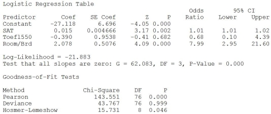 -Referring to Table 17-11,which of the following is the correct expression for the estimated model?
(Multiple Choice)
5.0/5 (44)
TABLE 17-2
One of the most common questions of prospective house buyers pertains to the cost of heating in dollars (Y).To provide its customers with information on that matter,a large real estate firm used the following 4 variables to predict heating costs: the daily minimum outside temperature in degrees of Fahrenheit (X1),the amount of insulation in inches (X2),the number of windows in the house (X3),and the age of the furnace in years (X4).Given below are the EXCEL outputs of two regression models.
-Referring to Table 17-2,the estimated value of the partial regression parameter β1in Model 1 means that
(Multiple Choice)
4.7/5 (43)
TABLE 17-10
Given below are results from the regression analysis where the dependent variable is the number of weeks a worker is unemployed due to a layoff (Unemploy)and the independent variables are the age of the worker (Age),the number of years of education received (Edu),the number of years at the previous job (Job Yr),a dummy variable for marital status (Married: 1 = married,0 = otherwise),a dummy variable for head of household (Head: 1 = yes,0 = no)and a dummy variable for management position (Manager: 1 = yes,0 = no).We shall call this Model 1.The coefficient of partial determination ( )of each of the 6 predictors are,respectively,0.2807,0.0386,0.0317,0.0141,0.0958,and 0.1201. Model 2 is the regression analysis where the dependent variable is Unemploy and the independent variables are Age and Manager.The results of the regression analysis are given below:
-Referring to Table 17-10,Model 1,predict the number of weeks being unemployed due to a layoff for a worker who is a thirty-year-old,has 10 years of education,has 15 years of experience at the previous job,is married,is the head of household and is a manager.
(Short Answer)
4.9/5 (30)
A researcher randomly sampled 30 graduates,18 males and 12 females,of an MBA program and recorded data concerning their starting salaries.Of primary interest to the researcher was the effect of gender on starting salaries.Statistics of the mean salaries of the females and males in the sample were computed.The sample standard deviations suggest that the variability of starting salaries of the two groups is almost the same.Suppose the starting salaries from both groups can be considered as normally distributed.Which of the following tests will be the most appropriate?
(Multiple Choice)
4.9/5 (43)
TABLE 17-10
Given below are results from the regression analysis where the dependent variable is the number of weeks a worker is unemployed due to a layoff (Unemploy)and the independent variables are the age of the worker (Age),the number of years of education received (Edu),the number of years at the previous job (Job Yr),a dummy variable for marital status (Married: 1 = married,0 = otherwise),a dummy variable for head of household (Head: 1 = yes,0 = no)and a dummy variable for management position (Manager: 1 = yes,0 = no).We shall call this Model 1.The coefficient of partial determination ( )of each of the 6 predictors are,respectively,0.2807,0.0386,0.0317,0.0141,0.0958,and 0.1201. Model 2 is the regression analysis where the dependent variable is Unemploy and the independent variables are Age and Manager.The results of the regression analysis are given below:
-Referring to Table 17-10,Model 1,what is the p-value of the test statistic when testing whether age has any effect on the number of weeks a worker is unemployed due to a layoff while holding constant the effect of all the other independent variables?
(Short Answer)
4.9/5 (35)
Filters
- Essay(0)
- Multiple Choice(0)
- Short Answer(0)
- True False(0)
- Matching(0)