Exam 14: Introduction to Multiple Regression

TABLE 14-15 The superintendent of a school district wanted to predict the percentage of students passing a sixth-grade proficiency test.She obtained the data on percentage of students passing the proficiency test (% Passing),mean teacher salary in thousands of dollars (Salaries),and instructional spending per pupil in thousands of dollars (Spending)of 47 schools in the state. Following is the multiple regression output with Y = % Passing as the dependent variable,X₁ = Salaries and X₂ = Spending: 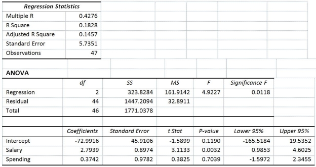-True or False: Referring to Table 14-15,you can conclude definitively that mean teacher salary individually has no impact on the mean percentage of students passing the proficiency test,taking into account the effect of instructional spending per pupil,at a 1% level of significance based solely on but not actually computing the 99% confidence interval estimate for β₁.

TABLE 14-1 A manager of a product sales group believes the number of sales made by an employee (Y)depends on how many years that employee has been with the company (X₁)and how he/she scored on a business aptitude test (X₂).A random sample of 8 employees provides the following: 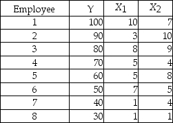-Referring to Table 14-1,if an employee who had been with the company 5 years scored a 9 on the aptitude test,what would his estimated expected sales be?

TABLE 14-13 An econometrician is interested in evaluating the relationship of demand for building materials to mortgage rates in Los Angeles and San Francisco.He believes that the appropriate model is Y = 10 + 5X₁ + 8X₂ where X₁ = mortgage rate in % X₂ = 1 if SF,0 if LA Y = demand in $100 per capita -Referring to Table 14-13,the predicted demand in San Francisco when the mortgage rate is 10% is ________.

TABLE 14-18 A logistic regression model was estimated in order to predict the probability that a randomly chosen university or college would be a private university using information on mean total Scholastic Aptitude Test score (SAT)at the university or college and whether the TOEFL criterion is at least 90 (Toefl90 = 1 if yes,0 otherwise).The dependent variable,Y,is school type (Type = 1 if private and 0 otherwise). The PHStat output is given below: 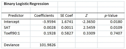-Referring to Table 14-18,what is the estimated probability that a school with a mean SAT score of 1100 and a TOEFL criterion that is not at least 90?

TABLE 14-7 The department head of the accounting department wanted to see if she could predict the GPA of students using the number of course units (credits)and total SAT scores of each.She takes a sample of students and generates the following Microsoft Excel output: 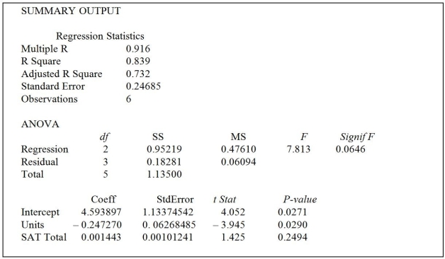-Referring to Table 14-7,the department head wants to test H₀ : β₁ = β₂ = 0.The critical value of the F test for a level of significance of 0.05 is ________.

TABLE 14-3 An economist is interested to see how consumption for an economy (in $ billions)is influenced by gross domestic product ($ billions)and aggregate price (consumer price index).The Microsoft Excel output of this regression is partially reproduced below. 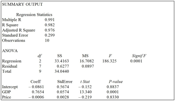-Referring to Table 14-3,to test for the significance of the coefficient on aggregate price index,the value of the relevant t-statistic is

TABLE 14-17 Given below are results from the regression analysis where the dependent variable is the number of weeks a worker is unemployed due to a layoff (Unemploy)and the independent variables are the age of the worker (Age)and a dummy variable for management position (Manager: 1 = yes,0 = no). The results of the regression analysis are given below: 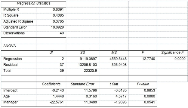-True or False: Referring to Table 14-17,the null hypothesis H₀ : β₁ = β₂ = 0 implies that the number of weeks a worker is unemployed due to a layoff is not related to any of the explanatory variables.

TABLE 14-8 A financial analyst wanted to examine the relationship between salary (in $1,000)and 2 variables: age (X₁ = Age)and experience in the field (X₂ = Exper).He took a sample of 20 employees and obtained the following Microsoft Excel output: 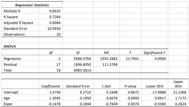Also,the sum of squares due to the regression for the model that includes only Age is 5022.0654 while the sum of squares due to the regression for the model that includes only Exper is 125.9848. -Referring to Table 14-8,the value of the partial F test statistic is ________ for H₀ : Variable X₂ does not significantly improve the model after variable X₁ has been included H₁ : Variable X₂ significantly improves the model after variable X₁ has been included

In a multiple regression model,which of the following is correct regarding the value of the adjusted r²?

TABLE 14-6 One of the most common questions of prospective house buyers pertains to the cost of heating in dollars (Y).To provide its customers with information on that matter,a large real estate firm used the following 2 variables to predict heating costs: the daily minimum outside temperature in degrees of Fahrenheit (X₁)and the amount of insulation in inches (X₂).Given below is EXCEL output of the regression model. 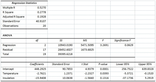Also SSR (X₁ ∣ X₂)= 8343.3572 and SSR (X₂ ∣ X₁)= 4199.2672 -True or False: A regression had the following results: SST = 102.55,SSE = 82.04.It can be said that 20.0% of the variation in the dependent variable is explained by the independent variables in the regression.

TABLE 14-4 A real estate builder wishes to determine how house size (House)is influenced by family income (Income)and family size (Size).House size is measured in hundreds of square feet and income is measured in thousands of dollars.The builder randomly selected 50 families and ran the multiple regression.Partial Microsoft Excel output is provided below: 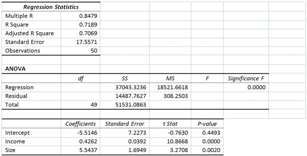Also SSR (X₁ ∣ X₂)= 36400.6326 and SSR (X₂ ∣ X₁)= 3297.7917 -Referring to Table 14-4,at the 0.01 level of significance,what conclusion should the builder reach regarding the inclusion of Income in the regression model?

TABLE 14-11 A weight-loss clinic wants to use regression analysis to build a model for weight loss of a client (measured in pounds).Two variables thought to affect weight loss are client's length of time on the weight-loss program and time of session.These variables are described below: Y = Weight loss (in pounds) X₁ = Length of time in weight-loss program (in months) X₂ = 1 if morning session,0 if not Data for 25 clients on a weight-loss program at the clinic were collected and used to fit the interaction model: Y = β₀ + β₁X₁ + β₂X₂ + β₃X₁X₂ + ε Output from Microsoft Excel follows: 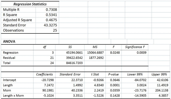-In a multiple regression model,the adjusted r²

TABLE 14-8 A financial analyst wanted to examine the relationship between salary (in $1,000)and 2 variables: age (X₁ = Age)and experience in the field (X₂ = Exper).He took a sample of 20 employees and obtained the following Microsoft Excel output: Also,the sum of squares due to the regression for the model that includes only Age is 5022.0654 while the sum of squares due to the regression for the model that includes only Exper is 125.9848. -True or False: Referring to Table 14-8,the F test for the significance of the entire regression performed at a level of significance of 0.01 leads to a rejection of the null hypothesis.

TABLE 14-4 A real estate builder wishes to determine how house size (House)is influenced by family income (Income)and family size (Size).House size is measured in hundreds of square feet and income is measured in thousands of dollars.The builder randomly selected 50 families and ran the multiple regression.Partial Microsoft Excel output is provided below: Also SSR (X₁ ∣ X₂)= 36400.6326 and SSR (X₂ ∣ X₁)= 3297.7917 -Referring to Table 14-4,what are the regression degrees of freedom that are missing from the output?

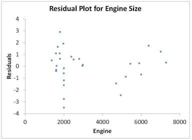
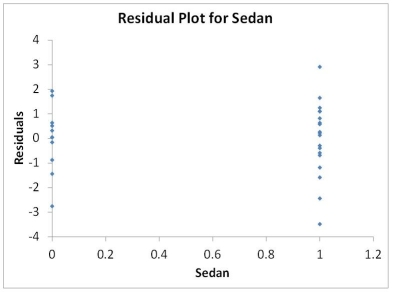
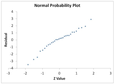
TABLE 14-16 What are the factors that determine the acceleration time (in sec.)from 0 to 60 miles per hour of a car? Data on the following variables for 30 different vehicle models were collected: Y (Accel Time): Acceleration time in sec. X₁ (Engine Size): c.c. X₂ (Sedan): 1 if the vehicle model is a sedan and 0 otherwise The regression results using acceleration time as the dependent variable and the remaining variables as the independent variables are presented below. 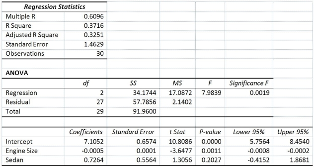The various residual plots are as shown below. 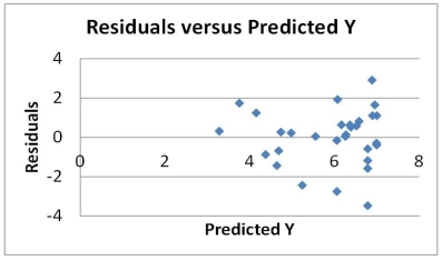The coefficient of partial determinations and are 0.3301,and 0.0594,respectively. The coefficient of determination for the regression model using each of the 2 independent variables as the dependent variable and the other independent variable as independent variables ( )are,respectively 0.0077,and 0.0077. -Referring to Table 14-16,________ of the variation in Accel Time can be explained by the two independent variables.

TABLE 14-17 Given below are results from the regression analysis where the dependent variable is the number of weeks a worker is unemployed due to a layoff (Unemploy)and the independent variables are the age of the worker (Age)and a dummy variable for management position (Manager: 1 = yes,0 = no). The results of the regression analysis are given below: -True or False: Referring to Table 14-17,the null hypothesis should be rejected at a 10% level of significance when testing whether there is a significant relationship between the number of weeks a worker is unemployed due to a layoff and the entire set of explanatory variables.

TABLE 14-15 The superintendent of a school district wanted to predict the percentage of students passing a sixth-grade proficiency test.She obtained the data on percentage of students passing the proficiency test (% Passing),mean teacher salary in thousands of dollars (Salaries),and instructional spending per pupil in thousands of dollars (Spending)of 47 schools in the state. Following is the multiple regression output with Y = % Passing as the dependent variable,X₁ = Salaries and X₂ = Spending: -Referring to Table 14-15,what are the lower and upper limits of the 95% confidence interval estimate for the effect of a one thousand dollar increase in instructional spending per pupil on the mean percentage of students passing the proficiency test?

TABLE 14-8 A financial analyst wanted to examine the relationship between salary (in $1,000)and 2 variables: age (X₁ = Age)and experience in the field (X₂ = Exper).He took a sample of 20 employees and obtained the following Microsoft Excel output: Also,the sum of squares due to the regression for the model that includes only Age is 5022.0654 while the sum of squares due to the regression for the model that includes only Exper is 125.9848. -Referring to Table 14-8,the predicted salary (in $1,000)for a 35-year-old person with 10 years of experience is ________.

TABLE 14-7 The department head of the accounting department wanted to see if she could predict the GPA of students using the number of course units (credits)and total SAT scores of each.She takes a sample of students and generates the following Microsoft Excel output: -True or False: Referring to Table 14-7,the department head wants to test H₀ : β₁ = β₂ = 0.At a level of significance of 0.05,the null hypothesis is rejected.

TABLE 14-11 A weight-loss clinic wants to use regression analysis to build a model for weight loss of a client (measured in pounds).Two variables thought to affect weight loss are client's length of time on the weight-loss program and time of session.These variables are described below: Y = Weight loss (in pounds) X₁ = Length of time in weight-loss program (in months) X₂ = 1 if morning session,0 if not Data for 25 clients on a weight-loss program at the clinic were collected and used to fit the interaction model: Y = β₀ + β₁X₁ + β₂X₂ + β₃X₁X₂ + ε Output from Microsoft Excel follows: -Referring to Table 14-11,what is the experimental unit for this analysis?