Exam 15: Multiple Regression Model Building

TABLE 15- 8 The superintendent of a school district wanted to predict the percentage of students passing a sixth- grade proficiency test. She obtained the data on percentage of students passing the proficiency test (% Passing), daily average of the percentage of students attending class (% Attendance), average teacher salary in dollars (Salaries), and instructional spending per pupil in dollars (Spending) of 47 schools in the state. Let Y = % Passing as the dependent variable, X₁ = % Attendance, X₂ = Salaries and X₃ = Spending. The coefficient of multiple determination (R ² _j) of each of the 3 predictors with all the other remaining predictors are,respectively, 0.0338, 0.4669, and 0.4743. The output from the best- subset regressions is given below: Adjusted Model Variables R Square R Square Std. 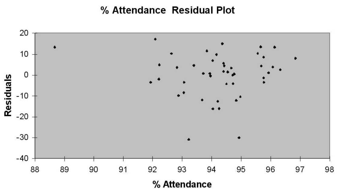Error 1 X1 3.05 2 0.6024 0.5936 10.5787 2 X1X2 3.66 3 0.6145 0.5970 10.5350 3 X1X2X3 4.00 4 0.6288 0.6029 10.4570 4 X1X3 2.00 3 0.6288 0.6119 10.3375 5 X2 67.35 2 0.0474 0.0262 16.3755 6 X2X3 64.30 3 0.0910 0.0497 16.1768 7 X3 62.33 2 0.0907 0.0705 15.9984 Following is the residual plot for % Attendance: Following is the output of several multiple regression models: $\text {Model (I):}$ Coefficients Std Error Stat p-value Lower 95\% Upper 95\% Intercept -753.4225 101.1149 -7.4511 2.88-09 -957.3401 -549.5050 \% Attend 8.5014 1.0771 7.8929 6.73-10 6.3292 10.6735 Salary 6.85-07 0.0006 0.0011 0.9991 -0.0013 0.0013 Spending 0.0060 0.0046 1.2879 0.2047 -0.0034 0.0153 $\text {Model (II):}$ Coefficients Standard Error t Stat p -value Intercept -753.4086 99.1451 -7.5991 1.5291-09 \% Attendance 8.5014 1.0645 7.9862 4.223-10 Spending 0.0060 0.0034 1.7676 0.0840 $\text {Model (III):}$ d f SS MS F Significance F Regression 2 8162.9429 4081.4714 39.8708 1.3201-10 Residual 44 4504.1635 102.3674 Total 46 12667.1064 Coefficients Standard Error t Stat p -value Intercept 6672.8367 3267.7349 2.0420 0.0472 \% Attendance -150.5694 69.9519 -2.1525 0.0369 \% Attendance Squared 0.8532 0.3743 2.2792 0.0276 -Referring to Table 15-8, the "best" model using a 5% level of significance among those chosen by the C_p statistic is

TABLE 15-3 A certain type of rare gem serves as a status symbol for many of its owners. In theory, for low prices, the demand increases and it decreases as the price of the gem increases. However, experts hypothesize that when the gem is valued at very high prices, the demand increases with price due to the status owners believe they gain in obtaining the gem. Thus, the model proposed to best explain the demand for the gem by its price is the quadratic model: $Y=\beta_{0}+\beta_{1} X+\beta_{2} X^{2}+\varepsilon$ where Y = demand (in thousands) and X = retail price per carat. This model was fit to data collected for a sample of 12 rare gems of this type. A portion of the computer analysis obtained from Microsoft Excel is shown below: SUMMARY OUTPUT Regression Statistics Multiple R 0.994 R Square 0.988 Standard Error 12.42 Observations 12 $\text { ANOVA }$ df SS MS F Signifcance F Regression 2 115145 57573 373 0.0001 Residual 9 1388 154 Total 11 116533 Coeff Std Error t Stat p-value Intercept 286.42 9.66 29.64 0.0001 Price -0.31 0.06 -5.14 0.0006 Frice Sq 0.000067 0.00007 0.95 0.3647 -Referring to Table 15-3, what is the p-value associated with the test statistic for testing whether there is an upward curvature in the response curve relating the demand (Y) and the price (X)?

Which of the following is used to determine observations that have influential effect on the fitted model?

TABLE 15-1 To explain personal consumption (CONS) measured in dollars, data is collected for $\text {INC: personal income indollars}$ $\quad$$\quad$$\text {CRDTLIM: \$ 1 plus the credit limit in dollars}$ $\quad$$\quad$$\text { available to the individual }$ $\quad$$\quad$$\text {APR: average annualized percentage interest rate for}$ $\quad$$\text { borrowing for the individual}$ $\text {ADVT: perperson advertisingexpenditure}$ $\quad$$\quad$$\quad$$\text { in dollars by manufacturers in the}$ $\quad$$\quad$$\quad$ $\text {city where the individual lives}$ $\text { SEX: gender of the individual: 1 if female, 0 if male}$ A regression analysis was performed with CONS as the dependent variable and ln(CRDTLIM), ln(APR), ln(ADVT), and SEX as the independent variables. The estimated model was y^{^} = 2.28 - 0.29 ln(CRDTLIM) + 5.77 ln(APR) + 2.35 ln(ADVT) + 0.39 SEX -Referring to Table 15-1, what is the correct interpretation for the estimated coefficient for ADVT?

TABLE 15-7 A chemist employed by a pharmaceutical firm has developed a muscle relaxant. She took a sample of 14 people suffering from extreme muscle constriction. She gave each a vial containing a dose (X) of the drug and recorded the time to relief (Y) measured in seconds for each. She fit a "centered" curvilinear model to this data. The results obtained by Microsoft Excel follow, where the dose (X) given has been "centered." SUMMARY OUTPUT Regression Statistics Multiple R 0.747 RSquare 0.558 Adjusted R Square 0.478 Standard Error 863.1 Observations 14 ANOVA df SS MS F Significance F Regression 2 10344797 5172399 6.94 0.0110 Residual 11 8193929 744903 Total 13 18538726 Coeff Std Error t Stut p -value Intercept 1283.0 352.0 3.65 0.0040 CenDose 25.228 8.631 2.92 0.0140 CenDoseSq 0.8604 0.3722 2.31 0.0410 -Referring to Table 15-7, suppose the chemist decides to use a t test to determine if there is a significant difference between a linear model and a curvilinear model that includes a linear term. If she used a level of significance of 0.02, she would decide that the linear model is sufficient.

Which of the following will not change a nonlinear model into a linear model?

The stepwise regression approach takes into consideration all possible models.

TABLE 15- 8 The superintendent of a school district wanted to predict the percentage of students passing a sixth- grade proficiency test. She obtained the data on percentage of students passing the proficiency test (% Passing), daily average of the percentage of students attending class (% Attendance), average teacher salary in dollars (Salaries), and instructional spending per pupil in dollars (Spending) of 47 schools in the state. Let Y = % Passing as the dependent variable, X₁ = % Attendance, X₂ = Salaries and X₃ = Spending. The coefficient of multiple determination (R ² _j) of each of the 3 predictors with all the other remaining predictors are, respectively, 0.0338, 0.4669, and 0.4743. The output from the best- subset regressions is given below: Adjusted Following is the residual plot for % Attendance: Adjusted Model Variables R Square R Square Std. Error 1 X1 3.05 2 0.6024 0.5936 10.5787 2 X1X2 3.66 3 0.6145 0.5970 10.5350 3 X1X2X3 4.00 4 0.6288 0.6029 10.4570 4 X1X3 2.00 3 0.6288 0.6119 10.3375 5 X2 67.35 2 0.0474 0.0262 16.3755 6 X2X3 64.30 3 0.0910 0.0497 16.1768 7 X3 62.33 2 0.0907 0.0705 15.9984 Following is the residual plot for % Attendance: Following is the output of several multiple regression models: $\text {Model (I):}$ Coefficients Std Error Stat p-value Lower 95\% Upper 95\% Intercept -753.4225 101.1149 -7.4511 2.88-09 -957.3401 -549.5050 \% Attend 8.5014 1.0771 7.8929 6.73-10 6.3292 10.6735 Salary 6.85-07 0.0006 0.0011 0.9991 -0.0013 0.0013 Spending 0.0060 0.0046 1.2879 0.2047 -0.0034 0.0153 $\text {Model (II):}$ Coefficients Standard Error t Stat p -value Intercept -753.4086 99.1451 -7.5991 1.5291-09 \% Attendance 8.5014 1.0645 7.9862 4.223-10 Spending 0.0060 0.0034 1.7676 0.0840 $\text {Model (III):}$ d f SS MS F Significance F Regression 2 8162.9429 4081.4714 39.8708 1.3201-10 Residual 44 4504.1635 102.3674 Total 46 12667.1064 Coefficients Standard Error t Stat p -value Intercept 6672.8367 3267.7349 2.0420 0.0472 \% Attendance -150.5694 69.9519 -2.1525 0.0369 \% Attendance Squared 0.8532 0.3743 2.2792 0.0276 -Referring to Table 15-8, there is reason to suspect collinearity between some pairs of predictors.