Exam 13: Simple Linear Regression

TABLE 13-7 An investment specialist claims that if one holds a portfolio that moves in the opposite direction to the market index like the S&P 500, then it is possible to reduce the variability of the portfolio's return. In other words, one can create a portfolio with positive returns but less exposure to risk. A sample of 26 years of S&P 500 index and a portfolio consisting of stocks of private prisons, which are believed to be negatively related to the S&P 500 index, is collected. A regression analysis was performed by regressing the returns of the prison stocks portfolio (Y) on the returns of S&P 500 index (X) to prove that the prison stocks portfolio is negatively related to the S&P 500 index at a 5% level of significance. The results are given in the following EXCEL output. Coefficients Standard Enor T Stat p -value Intercept 4.866004258 0.35743609 13.61363441 8.7932-13 S\&P -0.502513506 0.071597152- 7.01862425 2.94942-07 -Referring to Table 13-7, which of the following will be a correct conclusion?

TABLE 13-4 The managers of a brokerage firm are interested in finding out if the number of new clients a broker brings into the firm affects the sales generated by the broker. They sample 12 brokers and determine the number of new clients they have enrolled in the last year and their sales amounts in thousands of dollars. These data are presented in the table that follows. Broker Clients Sales 1 27 52 2 11 37 3 42 64 4 33 55 5 15 29 6 15 34 7 25 58 8 36 59 9 28 44 10 30 48 11 17 31 12 22 38 -Referring to Table 13-4, the regression sum of squares (SSR) is _______.

The residual represents the discrepancy between the observed dependent variable and its______value.

TABLE 13-01 A large national bank charges local companies for using their services. A bank official reported the results of a regression analysis designed to predict the bank's charges (Y) -- measured in dollars per month -- for services rendered to local companies. One independent variable used to predict service charge to a company is the company's sales revenue (X) -- measured in millions of dollars. Data for 21 companies who use the bank's services were used to fit the model: $E(Y)=\beta_{0}+\beta_{1} X$ The results of the simple linear regression are provided below. $\hat{Y}=-2,700+20 X, \mathrm{~S}_{Y X}=65, \text { two-tailed } p \text { value }=0.034\left(\text { for testing } \beta_{1}\right)$ -Referring to Table 13-1, interpret the p-value for testing whether þ1 exceeds 0.

TABLE 13-10 The management of a chain electronic store would like to develop a model for predicting the weekly sales (in thousand of dollars) for individual stores based on the number of customers who made purchases. A random sample of 12 stores yields the following results: Customers Sales (Thousands of Dollars) 907 11.20 926 11.05 713 8.21 741 9.21 780 9.42 898 10.08 510 6.73 529 7.02 460 6.12 872 9.52 650 7.53 603 7.25 -Referring to Table 13-10, what is the p-value of the F test statistic when testing whether the number of customers who make purchases is a good predictor for weekly sales?

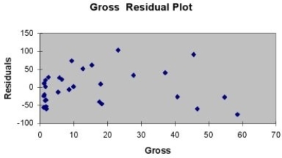
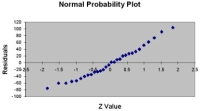
TABLE 13- 11 A company that has the distribution rights to home video sales of previously released movies would like to use the box office gross (in millions of dollars) to estimate the number of units (in thousands of units) that it can expect to sell. Following is the output from a simple linear regression along with the residual plot and normal probability plot obtained from a data set of 30 different movie titles: Regression Statistics Multiple R 0.8531 RSquare 0.7278 Adjusted R Square 0.7180 Standard Error 47.8668 Observations 30 ANOVA d f SS MS F Significance F Regression 1 171499.78 171499.78 74.8505 2.1259E-09 Residual 28 64154.42 2291.23 Total 29 235654.20 Coefficients Standard Error t Stat p -value Lower 95\% Upper 95\% Intercept 76.5351 11.8318 6.4686 5.24-07 52.2987 100.7716 Gross 4.3331 0.5008 8.6516 2.13-09 3.3072 5.3590 -Referring to Table 13-11, what is the value of the test statistic for testing whether there is a linear relationship between box office gross and home video unit sales?

TABLE 13-10 The management of a chain electronic store would like to develop a model for predicting the weekly sales (in thousand of dollars) for individual stores based on the number of customers who made purchases. A random sample of 12 stores yields the following results: Customers Sales (Thousands of Dollars) 907 11.20 926 11.05 713 8.21 741 9.21 780 9.42 898 10.08 510 6.73 529 7.02 460 6.12 872 9.52 650 7.53 603 7.25 -Referring to Table 13-10, what is the p-value of the t test statistic when testing whether the number of customers who make purchase affects weekly sales?

TABLE 13-2 A candy bar manufacturer is interested in trying to estimate how sales are influenced by the price of their product. To do this, the company randomly chooses 6 small cities and offers the candy bar at different prices. Using candy bar sales as the dependent variable, the company will conduct a simple linear regression on the data below: City Price (\ ) Sales River Falls 1.30 100 Hudson 1.60 90 Ellsworth 1.80 90 Prescott 2.00 40 Rock Elm 2.40 38 Stillwater 2.90 32 -Referring to Table 13-2, what is the standard error of the regression slope estimate, S_b1?

TABLE 13- 11 A company that has the distribution rights to home video sales of previously released movies would like to use the box office gross (in millions of dollars) to estimate the number of units (in thousands of units) that it can expect to sell. Following is the output from a simple linear regression along with the residual plot and normal probability plot obtained from a data set of 30 different movie titles: Regression Statistics Multiple R 0.8531 RSquare 0.7278 Adjusted R Square 0.7180 Standard Error 47.8668 Observations 30 ANOVA d f SS MS F Significance F Regression 1 171499.78 171499.78 74.8505 2.1259E-09 Residual 28 64154.42 2291.23 Total 29 235654.20 Coefficients Standard Error t Stat p -value Lower 95\% Upper 95\% Intercept 76.5351 11.8318 6.4686 5.24-07 52.2987 100.7716 Gross 4.3331 0.5008 8.6516 2.13-09 3.3072 5.3590 -Referring to Table 13-11, there is sufficient evidence that box office gross and home video unit sales are linearly related at a 5% level of significance.

TABLE 13- 11 A company that has the distribution rights to home video sales of previously released movies would like to use the box office gross (in millions of dollars) to estimate the number of units (in thousands of units) that it can expect to sell. Following is the output from a simple linear regression along with the residual plot and normal probability plot obtained from a data set of 30 different movie titles: Regression Statistics Multiple R 0.8531 RSquare 0.7278 Adjusted R Square 0.7180 Standard Error 47.8668 Observations 30 ANOVA d f SS MS F Significance F Regression 1 171499.78 171499.78 74.8505 2.1259E-09 Residual 28 64154.42 2291.23 Total 29 235654.20 Coefficients Standard Error t Stat p -value Lower 95\% Upper 95\% Intercept 76.5351 11.8318 6.4686 5.24-07 52.2987 100.7716 Gross 4.3331 0.5008 8.6516 2.13-09 3.3072 5.3590 -Referring to Table 13-11, which of the following is the correct interpretation for the coefficient of determination?

TABLE 13- 11 A company that has the distribution rights to home video sales of previously released movies would like to use the box office gross (in millions of dollars) to estimate the number of units (in thousands of units) that it can expect to sell. Following is the output from a simple linear regression along with the residual plot and normal probability plot obtained from a data set of 30 different movie titles: Regression Statistics Multiple R 0.8531 R Square 0.7278 Adjusted R Square 0.7180 Standard Error 47.8668 Observations 30 ANOVA d f SS MS F Significance F Regression 1 171499.78 171499.78 74.8505 2.1259E-09 Residual 28 64154.42 2291.23 Total 29 235654.20 Coefficients Standard Error t Stat p -value Lower 95\% Upper 95\% Intercept 76.5351 11.8318 6.4686 5.24-07 52.2987 100.7716 Gross 4.3331 0.5008 8.6516 2.13-09 3.3072 5.3590 -Referring to Table 13-11, predict the video unit sales for a movie that had a box office gross of $30 millions.

TABLE 13-3 The director of cooperative education at a state college wants to examine the effect of cooperative education job experience on marketability in the work place. She takes a random sample of 4 students. For these 4, she finds out how many times each had a cooperative education job and how many job offers they received upon graduation. These data are presented in the table below. Student CoopJobs JobOffer 1 1 4 2 2 6 3 1 3 4 0 1 -Referring to Table 13-3, the standard error of estimate is ______.

TABLE 13- 11 A company that has the distribution rights to home video sales of previously released movies would like to use the box office gross (in millions of dollars) to estimate the number of units (in thousands of units) that it can expect to sell. Following is the output from a simple linear regression along with the residual plot and normal probability plot obtained from a data set of 30 different movie titles: Regression Statistics Multiple R 0.8531 R Square 0.7278 Adjusted R Square 0.7180 Standard Error 47.8668 Observations 30 ANOVA d f SS MS F Significance F Regression 1 171499.78 171499.78 74.8505 2.1259E-09 Residual 28 64154.42 2291.23 Total 29 235654.20 Coefficients Standard Error t Stat p -value Lower 95\% Upper 95\% Intercept 76.5351 11.8318 6.4686 5.24-07 52.2987 100.7716 Gross 4.3331 0.5008 8.6516 2.13-09 3.3072 5.3590 -Referring to Table 13-11, what is the critical value for testing whether there is a linear relationship between box office gross and home video unit sales at a 5% level of significance?

TABLE 13-4 The managers of a brokerage firm are interested in finding out if the number of new clients a broker brings into the firm affects the sales generated by the broker. They sample 12 brokers and determine the number of new clients they have enrolled in the last year and their sales amounts in thousands of dollars. These data are presented in the table that follows. Broker Clients Sales 1 27 52 2 11 37 3 42 64 4 33 55 5 15 29 6 15 34 7 25 58 8 36 59 9 28 44 10 30 48 11 17 31 12 22 38 -Referring to Table 13-4, the managers of the brokerage firm wanted to test the hypothesis that the number of new clients brought in had a positive impact on the amount of sales generated. The value of the test statistic is ______.

You give a pre-employment examination to your applicants. The test is scored from 1 to 100. You have data on their sales at the end of one year measured in dollars. You want to know if there is any linear relationship between pre-employment examination score and sales. An appropriate test to use is the t test on the population correlation coefficient.

TABLE 13-4 The managers of a brokerage firm are interested in finding out if the number of new clients a broker brings into the firm affects the sales generated by the broker. They sample 12 brokers and determine the number of new clients they have enrolled in the last year and their sales amounts in thousands of dollars. These data are presented in the table that follows. Broker Clients Sales 1 27 52 2 11 37 3 42 64 4 33 55 5 15 29 6 15 34 7 25 58 8 36 59 9 28 44 10 30 48 11 17 31 12 22 38 -Referring to Table 13-4, the managers of the brokerage firm wanted to test the hypothesis that the true slope was equal to 0. The denominator of the test statistic is Sb1. The value of Sb1 in this sample is______ .