Exam 7: Hypothesis Tests and Confidence Intervals in Multiple Regression
Exam 1: Economic Questions and Data11 Questions
Exam 2: Review of Probability61 Questions
Exam 3: Review of Statistics56 Questions
Exam 4: Linear Regression With One Regressor54 Questions
Exam 5: Regression With a Single Regressor: Hypothesis Tests and Confidence Intervals53 Questions
Exam 6: Linear Regression With Multiple Regressors54 Questions
Exam 7: Hypothesis Tests and Confidence Intervals in Multiple Regression50 Questions
Exam 8: Nonlinear Regression Functions53 Questions
Exam 9: Assessing Studies Based on Multiple Regression55 Questions
Exam 10: Regression With Panel Data40 Questions
Exam 11: Regression With a Binary Dependent Variable40 Questions
Exam 12: Instrumental Variables Regression40 Questions
Exam 13: Experiments and Quasi-Experiments40 Questions
Exam 14: Introduction to Time Series Regression and Forecasting36 Questions
Exam 15: Estimation of Dynamic Causal Effects40 Questions
Exam 16: Additional Topics in Time Series Regression40 Questions
Exam 17: The Theory of Linear Regression With One Regressor39 Questions
Exam 18: The Theory of Multiple Regression38 Questions
Select questions type
Explain carefully why testing joint hypotheses simultaneously, using the F-statistic, does
not necessarily yield the same conclusion as testing them sequentially ("one at a time"
method), using a series of t-statistics.
(Essay)
4.8/5  (33)
(33)
Your textbook has emphasized that testing two hypothesis sequentially is not the same as testing them simultaneously. Consider the following confidence set below, where you are testing the hypothesis that .
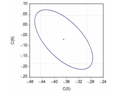 Your statistical package has also generated a dotted area, which corresponds to drawing
two confidence intervals for the respective coefficients.For each case where the ellipse
does not coincide in area with the corresponding rectangle, indicate what your decision
would be if you relied on the two confidence intervals vs.the ellipse generated by the F-
statistic.
Your statistical package has also generated a dotted area, which corresponds to drawing
two confidence intervals for the respective coefficients.For each case where the ellipse
does not coincide in area with the corresponding rectangle, indicate what your decision
would be if you relied on the two confidence intervals vs.the ellipse generated by the F-
statistic.
(Essay)
4.8/5 (47)
When there are two coefficients, the resulting confidence sets are
(Multiple Choice)
5.0/5 (32)
The confidence interval for a single coefficient in a multiple regression a. makes little sense because the population parameter is unknown.
b. should not be computed because there are other coefficients present in the model.
c. contains information from a large number of hypothesis tests.
d. should only be calculated if the regression is identical to the adjusted .
(Short Answer)
4.8/5 (35)
The homoskedasticity-only F-statistic is given by the following formula a. .
b. .
c. .
d. .
(Short Answer)
4.7/5 (38)
A subsample from the Current Population Survey is taken, on weekly earnings of
individuals, their age, and their gender.You have read in the news that women make 70
cents to the $1 that men earn.To test this hypothesis, you first regress earnings on a
constant and a binary variable, which takes on a value of 1 for females and is 0 otherwise.
The results were: = 570.70-170.72\times Female ,=0.084, SER =282.12. (9.44)(13.52)
(a)Perform a difference in means test and indicate whether or not the difference in the mean
salaries is significantly different.Justify your choice of a one-sided or two-sided
alternative test.Are these results evidence enough to argue that there is discrimination
against females? Why or why not? Is it likely that the errors are normally distributed in
this case? If not, does that present a problem to your test?
(Essay)
4.9/5 (34)
The following linear hypothesis can be tested using the F-test with the exception of a. and .
b. .
c. and .
d. and .
(Short Answer)
4.9/5 (39)
The administration of your university/college is thinking about implementing a policy of
coed floors only in dormitories.Currently there are only single gender floors.One reason
behind such a policy might be to generate an atmosphere of better "understanding"
between the sexes.The Dean of Students (DoS)has decided to investigate if such a
behavior results in more "togetherness" by attempting to find the determinants of the
gender composition at the dinner table in your main dining hall, and in that of a
neighboring university, which only allows for coed floors in their dorms.The survey
includes 176 students, 63 from your university/college, and 113 from a neighboring
institution.
The Dean's first problem is how to define gender composition.To begin with, the survey
excludes single persons' tables, since the study is to focus on group behavior.The Dean
also eliminates sports teams from the analysis, since a large number of single-gender
students will sit at the same table.Finally, the Dean decides to only analyze tables with
three or more students, since she worries about "couples" distorting the results.The Dean
finally settles for the following specification of the dependent variable: GenderComp of Male Students at Table
Where " " stands for absolute value of . The variable can take on values from zero to fifty. After considering various explanatory variables, the Dean settles for an initial list of
eight, and estimates the following relationship, using heteroskedasticity-robust standard
errors (this Dean obviously has taken an econometrics course earlier in her career and/or
has an able research assistant): =30.90-3.78\times Size -8.81\times DCoed +2.28\times DFemme +2.06\times DRoommate (7.73)(0.63)(2.66)(2.42)(2.39) -0.17\times DAthlete +1.49\times DCons -0.81 SAT +1.74\times SibOther, =0.24,=15.50 (3.23)(1.10)(1.20)(1.43) where Size is the number of persons at the table minus 3, DCoed is a binary variable,
which takes on the value of 1 if you live on a coed floor, DFemme is a binary variable,
which is 1 for females and zero otherwise, DRoommate is a binary variable which equals
1 if the person at the table has a roommate and is zero otherwise, DAthlete is a binary
variable which is 1 if the person at the table is a member of an athletic varsity team,
DCons is a variable which measures the political tendency of the person at the table on a
seven-point scale, ranging from 1 being "liberal" to 7 being "conservative," SAT is the
SAT score of the person at the table measured on a seven-point scale, ranging from 1 for
the category "900-1000" to 7 for the category "1510 and above," and increasing by one
for 100 point increases, and SibOther is the number of siblings from the opposite gender
in the family the person at the table grew up with.
(a)Indicate which of the coefficients are statistically significant.
(Essay)
4.8/5 (35)
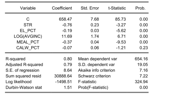
Consider the following regression output for an unrestricted and a restricted model. Unrestricted model:
Dependent Variable: TESTSCR
Method: Least Squares
Date: 07/31/06 Time: 17:35
Sample: 1420
Included observations: 420
 Restricted model:
Dependent Variable: TESTSCR
Method: Least Squares
Date: 07/31/06 Time: 17:37
Sample: 1420
Included observations: 420
Restricted model:
Dependent Variable: TESTSCR
Method: Least Squares
Date: 07/31/06 Time: 17:37
Sample: 1420
Included observations: 420
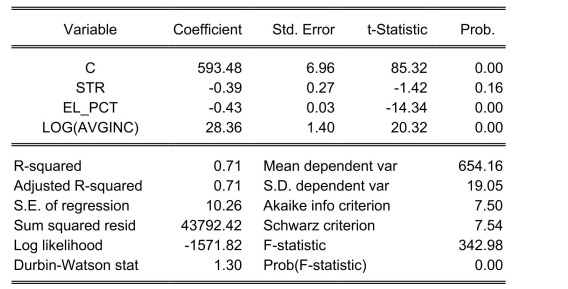 Calculate the homoskedasticity only F-statistic and determine whether the null hypothesis
can be rejected at the 5% significance level.
Calculate the homoskedasticity only F-statistic and determine whether the null hypothesis
can be rejected at the 5% significance level.
(Essay)
4.9/5 (36)
Set up the null hypothesis and alternative hypothesis carefully for the following cases:
(a)k = 4, test for all coefficients other than the intercept to be zero
(Essay)
4.7/5 (48)
You have estimated the following regression to explain hourly wages, using a sample of
250 individuals: = -2.44-1.57\times DFemme +0.27\times DMarried +0.59\times Educ +0.04\times Exper -0.60\times DNonwhite (1.29)(0.33)(0.36)(0.09)(0.01)(0.49) +0.13\times NCentral -0.11\times South (0.59)(0.58) =0.36,SER=2.74,n=250
Numbers in parenthesis are heteroskedasticity robust standard errors. Add "*" and "**" to indicate statistical significance of the coefficients.
(Essay)
4.9/5 (38)
You have estimated the following regression to explain hourly wages, using a sample of
250 individuals: = -2.44-1.57\times DFemme +0.27\times DMarried +0.59\times Educ +0.04\times Exper -0.60\times DNonwhite (1.29)(0.33)(0.36)(0.09)(0.01)(0.49) +0.13\times NCentral -0.11\times South (0.59)(0.58) =0.36,SER=2.74,n=250
Test the null hypothesis that the coefficients on DMarried, DNonwhite, and the two regional variables, NCentral and South are zero. The -statistic for the null hypothesis is . Do you reject the null hypothesis?
(Essay)
4.8/5 (36)
Let be 0.4366 and 0.4149 respectively. The difference between the unrestricted and the restricted model is that you have imposed two restrictions. There are 420 observations. The F -statistic in this case is
(Multiple Choice)
4.9/5 (46)
All of the following are examples of joint hypotheses on multiple regression coefficients, with the exception of a. .
b. and .
c. and .
d. and .
(Short Answer)
4.9/5 (28)
You have collected data for 104 countries to address the difficult questions of the
determinants for differences in the standard of living among the countries of the world.
You recall from your macroeconomics lectures that the neoclassical growth model
suggests that output per worker (per capita income)levels are determined by, among
others, the saving rate and population growth rate.To test the predictions of this growth
model, you run the following regression: = 0.339-12.894\timesn+1.397\times,=0.621,SER=0.177 (0.068)(3.177)(0.229) where RelPersInc is GDP per worker relative to the United States, n is the average
population growth rate, 1980-1990, and sK is the average investment share of GDP from
1960 to1990 (remember investment equals saving).Numbers in parentheses are for
heteroskedasticity-robust standard errors.
(a)Calculate the t-statistics and test whether or not each of the population parameters are
significantly different from zero.
(Essay)
4.9/5 (44)
To calculate the homoskedasticity-only overall regression -statistic, you need to compare the with the . Consider the following output from a regression package, which reproduces the regression results of testscores on the studentteacher ratio, the percent of English learners, and the expenditures per student from your textbook:
Dependent Variable: TESTSCR
Method: Least Squares
Date: 07/30/06 Time: 17:55
Sample: 1420
Included observations: 420
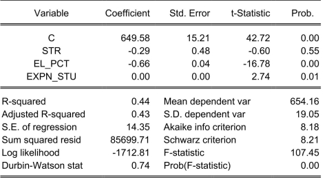 Sum of squared resid corresponds to . How are you going to find ? ii
(Essay)
4.7/5 (31)
Consider the following two models to explain testscores. Model 1:
Dependent Variable: TESTSCR
Method: Least Squares
Date: 07/31/06 Time: 17:52
Sample: 1420
Included observations: 420
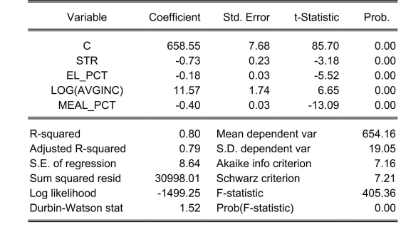 : Model 2:
Dependent Variable: TESTSCR
Method: Least Squares
Date: 07/31/06 Time: 17:56
Sample: 1420
Included observations: 420
: Model 2:
Dependent Variable: TESTSCR
Method: Least Squares
Date: 07/31/06 Time: 17:56
Sample: 1420
Included observations: 420
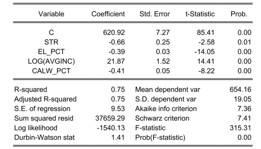 Explain why you cannot use the F-test in this situation to discriminate between Model 1
and Model 2.
Explain why you cannot use the F-test in this situation to discriminate between Model 1
and Model 2.
(Essay)
4.8/5 (41)
The homoskedasticity only F-statistic is given by the formula where is the sum of squared residuals from the restricted regression, is the sum of squared residuals from the unrestricted regression, is the number of restrictions under the null hypothesis, and is the number of regressors in the unrestricted regression. Prove that this formula is the same as the following formula based on the regression of the restricted and unrestricted regression:
(Essay)
4.8/5 (33)
Filters
- Essay(0)
- Multiple Choice(0)
- Short Answer(0)
- True False(0)
- Matching(0)