Exam 11: Simple Linear Regression
Exam 1: Statistics, Data, and Statistical Thinking73 Questions
Exam 2: Methods for Describing Sets of Data194 Questions
Exam 3: Probability283 Questions
Exam 4: Discrete Random Variables133 Questions
Exam 5: Continuous Random Variables139 Questions
Exam 6: Sampling Distributions47 Questions
Exam 7: Inferences Based on a Single Sample: Estimation With Confidence Intervals124 Questions
Exam 8: Inferences Based on a Single Sample: Tests of Hypothesis140 Questions
Exam 9: Inferences Based on a Two Samples: Confidence Intervals and Tests of Hypotheses94 Questions
Exam 10: Analysis of Variance: Comparing More Than Two Means90 Questions
Exam 11: Simple Linear Regression111 Questions
Exam 12: Multiple Regression and Model Building131 Questions
Exam 13: Categorical Data Analysis60 Questions
Exam 14: Nonparametric Statistics90 Questions
Select questions type
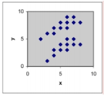
If a least squares line were determined for the data set in each scattergram, which would have the smallest variance? A)
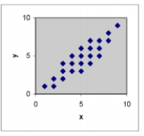 B)
B)
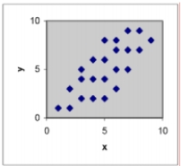 C)
C)
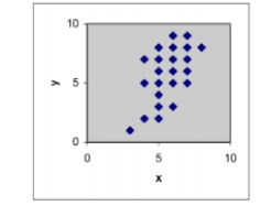 D)
D)
(Short Answer)
5.0/5  (38)
(38)
A study of the top 75 MBA programs attempted to predict the average starting salary (in $1000's) of graduates of the program based on the amount of tuition (in $1000's) charged by the program. The results of a simple linear regression analysis are shown below: Least Squares Linear Regression of Salary Predictor
Variables Coefficient Std Error T P Constant 18.1849 10.3336 1.76 0.0826 Size 1.47494 0.14017 10.52 0.0000
R-Squared Resid. Mean Square (MSE)
Adjusted R-Squared Standard Deviation In addition, we are told that the coefficient of correlation was calculated to be r = 0.7763. Interpret this result.
(Multiple Choice)
4.7/5 (28)
A manufacturer of boiler drums wants to use regression to predict the number of man-hours needed to erect drums in the future. The manufacturer collected a random sample of 35 boilers and measured the following two variables: MANHRS: Number of man-hours required to erect the drum
PRESSURE: Boiler design pressure (pounds per square inch, i.e., )
The simple linear model was fit to the data. A printout for the analysis appears below:
UNWEIGHTED LEAST SQUARES LINEAR REGRESSION OF MANHRS
PREDICTOR VARIABLES COEFFICIENT STD ERROR STUDENT'S T P CONSTANT 1.88059 0.58380 3.22 0.0028 PRESSURE 0.00321 0.00163 2.17 0.0300
R-SQUARED 0.4342 RESID. MEAN SQUARE (MSE) 4.25460 ADJUSTED R-SQUARED 0.4176 STANDARD DEVIATION 2.06267
SOURCE DF SS MS REGRESSION 1 111.008 111.008 5.19 0.0300 RESIDUAL 34 144.656 4.25160 TOTAL 35 255.665
Give a practical interpretation of the coefficient of determination, .
(Multiple Choice)
4.9/5 (18)
What is the relationship between diamond price and carat size? 307 diamonds were sampled and a straight-line relationship was hypothesized between y = diamond price (in dollars) and x = size of the diamond (in carats). The simple linear regression for the analysis is shown below: Least Squares Linear Regression of PRICE Predictor Variables Coefficient Std Error T P Constant -2298.36 158.531 -14.50 0.0000 Size 11598.9 230.111 50.41 0.0000 R-Squared 0.8925 Resid. Mean Square (MSE) 1248950 Adjusted R-Squared 0.8922 Standard Deviation 1117.56 The model was then used to create 95% confidence and prediction intervals for y and for E(Y) when the carat size of the diamond was 1 carat. The results are shown here: 95% confidence interval for E(Y): ($9091.60, $9509.40) 95% prediction interval for Y: ($7091.50, $11,510.00) Which of the following interpretations is correct if you want to use the model to estimate E(Y) for all 1-carat diamonds?
(Multiple Choice)
4.9/5 (42)
A breeder of Thoroughbred horses wishes to model the relationship between the gestation period and the length of life of a horse. The breeder believes that the two variables may follow a linear trend. The information in the table was supplied to the breeder from various thoroughbred stables across the state. Horse Gestation period Life Length Horse Gestation period Life Length 1 416 24 (years) x (days) y (years) 2 279 25.5 6 356 22 3 298 20 7 403 23.5 4 307 21.5 265 21 Summary statistics yield S=21,752,S=236.5,S=22,=332 , and =22.5 . Calculate SSE , s2, and s.
(Essay)
4.9/5 (31)
(Situation P) Below are the results of a survey of America's best graduate and professional schools. The top 25 business
schools, as determined by reputation, student selectivity, placement success, and graduation rate, are listed in the table.
For each school, three variables were measured: (1) GMAT score for the typical incoming student; (2) student acceptance
rate (percentage accepted of all students who applied); and (3) starting salary of the typical graduating student. School GMAT Acc. Rate Salary 1. Harvard 644 15.0\% \ 63,000 2. Stanford 665 10.2 60,000 3. Penn 644 19.4 55,000 4. Northwestern 640 22.6 54,000 5. MIT 650 21.3 57,000 6. Chicago 632 30.0 55,269 7. Duke 630 18.2 53,300 8. Dartmouth 649 13.4 52,000 9. Virginia 630 23.0 55,269 10. Michigan 620 32.4 53.300 11. Columbia 635 37.1 52,000 12. Cornell 648 14.9 50,700 13. CMU 630 31.2 52,050 14. UNC 625 15.4 50,800 15. Cal-Berkeley 634 24.7 50,000 16. UCLA 640 20.7 51,494 17. Texas 612 28.1 43,985 18. Indiana 600 29.0 44,119 19. NYU 610 35.0 53,161 20. Purdue 595 26.8 43,500 21. USC 610 31.9 49,080 22. Pittsburgh 605 33.0 43,500 23. Georgetown 617 31.7 45,156 24. Maryland 593 28.1 42,925 25. Rochester 605 35.9 44,499 The academic advisor wants to predict the typical starting salary of a graduate at a top business school using GMAT
score of the school as a predictor variable. A simple linear regression of SALARY versus GMAT using the 25 data points
in the table are shown below.
-For the situation above, write the equation of the probabilistic model of interest. A) Salary (GMAT)
B) Salary GMAT
C) GMAT (SALARY)
D) GMAT SALARY
(Short Answer)
4.9/5 (36)
(Situation P) Below are the results of a survey of America's best graduate and professional schools. The top 25 business
schools, as determined by reputation, student selectivity, placement success, and graduation rate, are listed in the table.
For each school, three variables were measured: (1) GMAT score for the typical incoming student; (2) student acceptance
rate (percentage accepted of all students who applied); and (3) starting salary of the typical graduating student. School GMAT Acc. Rate Salary 1. Harvard 644 15.0\% \ 63,000 2. Stanford 665 10.2 60,000 3. Penn 644 19.4 55,000 4. Northwestern 640 22.6 54,000 5. MIT 650 21.3 57,000 6. Chicago 632 30.0 55,269 7. Duke 630 18.2 53,300 8. Dartmouth 649 13.4 52,000 9. Virginia 630 23.0 55,269 10. Michigan 620 32.4 53.300 11. Columbia 635 37.1 52,000 12. Cornell 648 14.9 50,700 13. CMU 630 31.2 52,050 14. UNC 625 15.4 50,800 15. Cal-Berkeley 634 24.7 50,000 16. UCLA 640 20.7 51,494 17. Texas 612 28.1 43,985 18. Indiana 600 29.0 44,119 19. NYU 610 35.0 53,161 20. Purdue 595 26.8 43,500 21. USC 610 31.9 49,080 22. Pittsburgh 605 33.0 43,500 23. Georgetown 617 31.7 45,156 24. Maryland 593 28.1 42,925 25. Rochester 605 35.9 44,499 The academic advisor wants to predict the typical starting salary of a graduate at a top business school using GMAT
score of the school as a predictor variable. A simple linear regression of SALARY versus GMAT using the 25 data points
in the table are shown below.
-For the situation above, give a practical interpretation of
(Multiple Choice)
4.8/5 (34)
The dean of the Business School at a small Florida college wishes to determine whether the grade -point average (GPA) of a graduating student can be used to predict the graduate's starting salary. More specifically, the dean wants to know whether higher GPAs lead to higher starting salaries. Records for 23 of last year's Business School graduates are selected at random, and data on GPA (x) and starting salary (y, in $thousands) for each graduate were used to fit the model
The results of the simple linear regression are provided below.
=4.25+2.75x, SSxy=5.15,SSxx=1.87 SSyy=15.17,SSE=1.0075 Range of the x -values: 2.23-3.85 Range of the y -values: 9.3-15.6 Suppose a 95% prediction interval for y when x = 3.00 is (16, 21). Interpret the interval.
(Multiple Choice)
4.9/5 (35)
Consider the following model , where is the daily rate of return of a stock, and is the daily rate of return of the stock market as a whole, measured by the daily rate of return of Standard \& Poor's (S\&P) 500 Composite Index. Using a random sample of days from 1980 , the least squares lines shown in the table below were obtained for four firms. The estimated standard error of is shown to the right of each least squares prediction equation.
Firm Estimated Market Model Estimated Standard Error of Company A y=.0010+1.40x .03 Company B y=.0005-1.21x .06 Company C y=.0010+1.62x 1.34 Company D y=.0013+.76x .15
For which of the three stocks, Companies B, C, or D, is there evidence (at ) of a positive linear relationship between and ?
A) Company D only
B) Company C only
C) Companies B and C only
D) Companies B and D only
(Short Answer)
4.7/5 (34)
Is there a relationship between the raises administrators at State University receive and their performance on the job? A faculty group wants to determine whether job rating (x) is a useful linear predictor of raise (y). Consequently, the group considered the straight-line regression model
Using the method of least squares, the faculty group obtained the following prediction equation:
Interpret the estimated y-intercept of the line.
(Multiple Choice)
4.8/5 (33)
What is the relationship between diamond price and carat size? 307 diamonds were sampled and a straight-line relationship was hypothesized between y = diamond price (in dollars) and x = size of the diamond (in carats). The simple linear regression for the analysis is shown below: Least Squares Linear Regression of PRICE 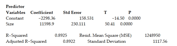 Interpret the estimated slope of the regression line.
(Multiple Choice)
4.9/5 (31)
State the four basic assumptions about the general form of the probability distribution of the random error ε.
(Essay)
4.8/5 (35)
An academic advisor wants to predict the typical starting salary of a graduate at a top business school using the GMAT score of the school as a predictor variable. A simple linear regression of SALARY versus GMAT using 25 data points is shown below.
Set up the null and alternative hypotheses for testing whether a linear relationship exists between SALARY and GMAT.
A) vs.
B) vs.
C) vs.
D) vs.
(Short Answer)
4.7/5 (36)
The dean of the Business School at a small Florida college wishes to determine whether the grade -point average (GPA) of a graduating student can be used to predict the graduate's starting salary. More specifically, the dean wants to know whether higher GPAs lead to higher starting salaries. Records for 23 of last year's Business School graduates are selected at random, and data on GPA (x) and starting salary (y, in $thousands) for each graduate were used to fit the model
The results of the simple linear regression are provided below.
=4.25+2.75x,S =5.15,S=1.87 S =15.17,SSE=1.0075 Compute an estimate of ?, the standard deviation of the random error term.
(Multiple Choice)
4.9/5 (33)
A county real estate appraiser wants to develop a statistical model to predict the appraised value of houses in a section of the county called East Meadow. One of the many variables thought to be an important predictor of appraised value is the number of rooms in the house. Consequently, the appraiser decided to fit the simple linear regression model:
where appraised value of the house (in thousands of dollars) and number of rooms. Using data collected for a sample of houses in East Meadow, the following results were obtained:
Give a practical interpretation of the estimate of ?, the standard deviation of the random error term in the model.
(Multiple Choice)
4.8/5 (34)
(Situation P) Below are the results of a survey of America's best graduate and professional schools. The top 25 business
schools, as determined by reputation, student selectivity, placement success, and graduation rate, are listed in the table.
For each school, three variables were measured: (1) GMAT score for the typical incoming student; (2) student acceptance
rate (percentage accepted of all students who applied); and (3) starting salary of the typical graduating student. School GMAT Acc. Rate Salary 1. Harvard 644 15.0\% \ 63,000 2. Stanford 665 10.2 60,000 3. Penn 644 19.4 55,000 4. Northwestern 640 22.6 54,000 5. MIT 650 21.3 57,000 6. Chicago 632 30.0 55,269 7. Duke 630 18.2 53,300 8. Dartmouth 649 13.4 52,000 9. Virginia 630 23.0 55,269 10. Michigan 620 32.4 53.300 11. Columbia 635 37.1 52,000 12. Cornell 648 14.9 50,700 13. CMU 630 31.2 52,050 14. UNC 625 15.4 50,800 15. Cal-Berkeley 634 24.7 50,000 16. UCLA 640 20.7 51,494 17. Texas 612 28.1 43,985 18. Indiana 600 29.0 44,119 19. NYU 610 35.0 53,161 20. Purdue 595 26.8 43,500 21. USC 610 31.9 49,080 22. Pittsburgh 605 33.0 43,500 23. Georgetown 617 31.7 45,156 24. Maryland 593 28.1 42,925 25. Rochester 605 35.9 44,499 The academic advisor wants to predict the typical starting salary of a graduate at a top business school using GMAT
score of the school as a predictor variable. A simple linear regression of SALARY versus GMAT using the 25 data points
in the table are shown below.
-For the situation above, give a practical interpretation of
(Multiple Choice)
4.8/5 (28)
A county real estate appraiser wants to develop a statistical model to predict the appraised value of houses in a section of the county called East Meadow. One of the many variables thought to be an important predictor of appraised value is the number of rooms in the house. Consequently, the appraiser decided to fit the simple linear regression model:
where appraised value of the house (in thousands of dollars) and number of rooms. Using data collected for a sample of houses in East Meadow, the following results were obtained:
What are the properties of the least squares line,
A) Average error of prediction is 0 , and is minimum.
B) It is normal, mean 0 , constant variance, and independent.
C) All 80 of the sample -values fall on the line.
D) It will always be a statistically useful predictor of .
(Short Answer)
4.8/5 (38)
What is the relationship between diamond price and carat size? 307 diamonds were sampled and a straight-line relationship was hypothesized between y = diamond price (in dollars) and x = size of the diamond (in carats). The simple linear regression for the analysis is shown below: Least Squares Linear Regression of PRICE 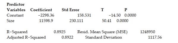 The model was then used to create 95% confidence and prediction intervals for y and for E(Y) when the carat size of the diamond was 1 carat. The results are shown here: 95% confidence interval for E(Y): ($9091.60, $9509.40) 95% prediction interval for Y: ($7091.50, $11,510.00) Which of the following interpretations is correct if you want to use the model to determine the price of a single 1-carat diamond?
(Multiple Choice)
4.8/5 (31)
Filters
- Essay(0)
- Multiple Choice(0)
- Short Answer(0)
- True False(0)
- Matching(0)