Exam 11: Simple Linear Regression

What is the relationship between diamond price and carat size? 307 diamonds were sampled (ranging in size from 0.18 to 1.1 carats) and a straight-line relationship was hypothesized between y = diamond price (in dollars) and x = size of the diamond (in carats). The simple linear regression for the analysis is shown below: Least Squares Linear Regression of PRICE 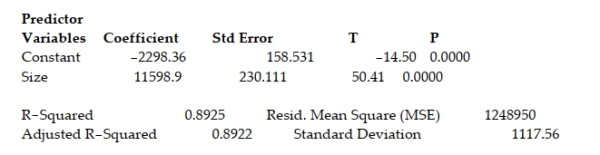Interpret the estimated y-intercept of the regression line.

A manufacturer of boiler drums wants to use regression to predict the number of man-hours needed to erect drums in the future. The manufacturer collected a random sample of 35 boilers and measured the following two variables: MANHRS: $\quad y =$ Number of man-hours required to erect the drum PRESSURE: $\quad x _ { 1 } =$ Boiler design pressure (pounds per square inch, i.e., $\mathrm { psi }$ ) The simple linear model $E ( y ) = \beta _ { 0 } + \beta _ { 1 } x$ was fit to the data. A printout for the analysis appears below: UNWEIGHTED LEAST SQUARES LINEAR REGRESSION OF MANHRS PREDICTOR VARIABLES COEFFICIENT STD ERROR STUDENT'S T P CONSTANT 1.88059 0.58380 3.22 0.0028 PRESSURE 0.00321 0.00163 2.17 0.0300 SOURCE DF SS MS REGRESSION 1 111.008 111.008 5.19 0.0300 RESIDUAL 34 144.656 4.25160 TOTAL 35 255.665 Fill in the blank. At ? =.01, there is ____________ between man-hours and pressure.

Plot the line y = 3x. Then give the slope and y-intercept of the line.

A large national bank charges local companies for using their services. A bank official reported the results of a regression analysis designed to predict the bank's charges (y), measured in dollars per month, for services rendered to local companies. One independent variable used to predict service charge to a company is the company's sales revenue (x), measured in $ million. Data for 21 companies who use the bank's services were used to fit the model $E ( y ) = \beta _ { 0 } + \beta _ { 1 } x .$ The results of the simple linear regression are provided below. $\hat { y } = 2,700 + 20 x , s = 65,2 \text {-tailed } p \text {-value } = .064 \text { (for testing } \beta _ { 1 } \text { ) }$ Interpret the $p$ -value for testing whether $\beta _ { 1 }$ exceeds 0 . A) There is sufficient evidence (at $\alpha = .05$ ) to conclude that service charge $( y )$ is positively linearly related to sales revenue $( x )$ . B) For every $\$ 1$ million increase in sales revenue $( x )$ , we expect a service charge $( y )$ to increase $\$ .064$ . C) There is insufficient evidence (at $\alpha = .05$ ) to conclude that service charge ( $y$ ) is positively linearly related to sales revenue $( x )$ . D) Sales revenue $( x )$ is a poor predictor of service charge $( y )$ .

What is the relationship between diamond price and carat size? 307 diamonds were sampled and a straight-line relationship was hypothesized between y = diamond price (in dollars) and x = size of the diamond (in carats). The simple linear regression for the analysis is shown below: Least Squares Linear Regression of PRICE Predictor Variables Coefficient Std Error T P Constant -2298.36 158.531 -14.50 0.0000 Size 11598.9 230.111 50.41 0.0000 R-Squared 0.8925 Resid. Mean Square (MSE) 1248950 Adjusted R-Squared 0.8922 Standard Deviation 1117.56 Interpret the coefficient of determination for the regression model.

Set up the null and alternative hypotheses for testing whether a positive linear relationship exists between SALARY and GMAT in the situation above. A) $H _ { 0 } : \beta _ { 1 } = 0$ vs. $H _ { a } : \beta _ { 1 } > 0$ B) $H _ { 0 } : \beta _ { 1 } = 0$ vs. $H _ { \mathrm { a } } : \beta _ { 1 } \neq 0$ C) $H _ { 0 } : \beta _ { 1 } = 228$ vs. $H _ { \mathrm { a } } : \beta _ { 1 } > 228$ D) $H _ { 0 } : \beta _ { 1 } > 0$ vs. $H _ { \mathrm { a } } : \beta _ { 1 } < 0$

Consider the data set shown below. Find the coefficient of determination for the simple linear regression model. 0 3 2 3 8 10 11 -2 0 2 4 6 8 10

In a study of feeding behavior, zoologists recorded the number of grunts of a warthog feeding by a lake in the 15 minute period following the addition of food. The data showing the number of grunts and and the age of the warthog (in days) are listed below: Number of Grunts Age (days) 93 128 71 144 42 158 47 163 66 170 43 177 65 186 20 192 23 198 Find and interpret the value of .

A large national bank charges local companies for using its services. A bank official reported the results of a regression analysis designed to predict the bank's charges (y), measured in dollars per month, for services rendered to local companies. One independent variable used to predict the service charge to a company is the company's sales revenue (x), measured in $ million. Data for 21 companies who use the bank's services were used to fit the model $E ( y ) = \beta _ { 0 } + \beta _ { 1 } x .$ The results of the simple linear regression are provided below. $\hat { y } = 2,700 + 20 x$ Interpret the estimate of $\beta _ { 0 }$ , the $y$ -intercept of the line.

An academic advisor wants to predict the typical starting salary of a graduate at a top business school using the GMAT score of the school as a predictor variable. A simple linear regression of SALARY versus GMAT using 25 data points is shown below. $\hat { \beta } _ { 0 } = - 92040 \hat { \beta } 1 = 228 s = 3213 r ^ { 2 } = .66 r = .81 \mathrm { df } = 23 \quad t = 6.67$ Give a practical interpretation of r = .81.

A high value of the correlation coefficient r implies that a causal relationship exists between x and y.

For the situation above, which of the following is not an assumption required for the simple linear regression analysis to be valid?

For the situation above, give a practical interpretation of t = 6.67.

a. Complete the table. yi 2 3 5 2 3 4 8 0 \Sigma= Totals \Sigma= \Sigma= \Sigma= b. Find $S S _ { x y } , S S _ { x x } , \beta _ { 1 } , \bar { x } , \bar { y }$ , and $\hat { \beta } _ { 0 }$ . c. Write the equation of the least squares line.

Is there a relationship between the raises administrators at State University receive and their performance on the job? A faculty group wants to determine whether job rating (x) is a useful linear predictor of raise (y). Consequently, the group considered the straight-line regression model $E ( y ) = \beta _ { 0 } + \beta _ { 1 } x .$ Using the method of least squares, the faculty group obtained the following prediction equation: $\hat { y } = 14,000 - 2,000 x$ Interpret the estimated slope of the line.

A county real estate appraiser wants to develop a statistical model to predict the appraised value of houses in a section of the county called East Meadow. One of the many variables thought to be an important predictor of appraised value is the number of rooms in the house. Consequently, the appraiser decided to fit the simple linear regression model: $E ( y ) = \beta _ { 0 } + \beta _ { 1 } x ,$ where $y =$ appraised value of the house (in thousands of dollars) and $x =$ number of rooms. Using data collected for a sample of $n = 74$ houses in East Meadow, the following restults were obtained: $\hat { y } = 74.80 + 21.66 x$ Give a practical interpretation of the estimate of the slope of the least squares line.

Is the number of games won by a major league baseball team in a season related to the team's batting average? Data from 14 teams were collected and the summary statistics yield: $\sum y = 1,134 , \sum x = 3.642 , \sum y ^ { 2 } = 93,110 , \sum x^ { 2 } = .948622 , \text { and } \sum x y = 295.54$ Assume $\hat { \beta } 1 = 455.27$ and $\hat { \sigma } = 9.18$ . Conduct a test of hypothesis to determine if a positive linear relationship exists between team batting average and number of wins. Use $\alpha = .05$ .

Plot the line y = 1.5 + .5x. Then give the slope and y-intercept of the line.

(Situation P) Below are the results of a survey of America's best graduate and professional schools. The top 25 business schools, as determined by reputation, student selectivity, placement success, and graduation rate, are listed in the table. For each school, three variables were measured: (1) GMAT score for the typical incoming student; (2) student acceptance rate (percentage accepted of all students who applied); and (3) starting salary of the typical graduating student. School GMAT Acc. Rate Salary 1. Harvard 644 15.0\% \ 63,000 2. Stanford 665 10.2 60,000 3. Penn 644 19.4 55,000 4. Northwestern 640 22.6 54,000 5. MIT 650 21.3 57,000 6. Chicago 632 30.0 55,269 7. Duke 630 18.2 53,300 8. Dartmouth 649 13.4 52,000 9. Virginia 630 23.0 55,269 10. Michigan 620 32.4 53.300 11. Columbia 635 37.1 52,000 12. Cornell 648 14.9 50,700 13. CMU 630 31.2 52,050 14. UNC 625 15.4 50,800 15. Cal-Berkeley 634 24.7 50,000 16. UCLA 640 20.7 51,494 17. Texas 612 28.1 43,985 18. Indiana 600 29.0 44,119 19. NYU 610 35.0 53,161 20. Purdue 595 26.8 43,500 21. USC 610 31.9 49,080 22. Pittsburgh 605 33.0 43,500 23. Georgetown 617 31.7 45,156 24. Maryland 593 28.1 42,925 25. Rochester 605 35.9 44,499 The academic advisor wants to predict the typical starting salary of a graduate at a top business school using GMAT score of the school as a predictor variable. A simple linear regression of SALARY versus GMAT using the 25 data points in the table are shown below. $\beta _ { 0 } = - 92040 \quad \hat { \beta } _ { 1 } = 228 \quad s = 3213 \quad r ^ { 2 } = .66 \quad r = .81 \quad \mathrm { df } = 23 \quad t = 6.67$ -For the situation above, give a practical interpretation of $r ^ { 2 } = .66$ . A) We expect to predict SALARY to within $2 ( \sqrt { .66 } )$ of its true value using GMAT in a straight-line model. B) We estimate SALARY to increase $\$ .66$ for every 1 -point increase in GMAT. C) $66 \%$ of the sample variation in SALARY can be explained by using GMAT in a straight -line model. D) We can predict SALARY correctly $66 \%$ of the time using GMAT in a straight-line model.

A company keeps extensive records on its new salespeople on the premise that sales should increase with experience. A random sample of seven new salespeople produced the data on experience and sales shown in the table. Months on Job Monthly Sales (\ thousands) 2 2.4 4 7.0 8 11.3 12 15.0 1 .8 5 3.7 9 12.0 Summary statistics yield $S S _ { x x } = 94.8571 , S S _ { x y } = 124.7571 , S S _ { y y } = 176.5171 , \bar { x } = 5.8571$ , and $\bar { y } = 7.4571$ . Calculate a $90 \%$ confidence interval for $E ( y )$ when $x = 5$ months. Assume $s = 1.577$ and the prediction equation is $\hat { y } = - .25 + 1.315 x$ .