Exam 12: Multiple Regression and Model Building

A collector of grandfather clocks believes that the price received for the clocks at an auction increases with the number of bidders, but at an increasing (rather than a constant) rate. Thus, the model proposed to best explain auction price (y, in dollars) by number of bidders (x) is the quadratic model $E ( y ) = \beta _ { 0 } + \beta _ { 1 } x + \beta _ { 2 } x ^ { 2 }$ This model was fit to data collected for a sample of 32 clocks sold at auction; a portion of the printout follows: PARAMETER STANDARD T FOR 0: VARIABLES ESTIMATE ERROR PARAMETER =0 PROB >|T| INTERCEPT 286.42 9.66 29.64 .0001 -.31 .06 -5.14 .0016 \cdot .000067 .00007 .95 .3600 Give the $p$ -value for testing $H _ { 0 } : \beta _ { 2 } = 0$ against $H _ { a } : \beta 2 \neq 0$ .

Retail price data for n = 60 hard disk drives were recently reported in a computer magazine. Three variables were recorded for each hard disk drive: $\mathrm { y } =$ Retail PRICE (measured in dollars) $\mathrm { x } _ { 1 } =$ Microprocessor SPEED (measured in megahertz) (Values in sample range from 10 to 40 ) $x _ { 2 } =$ CHIP size (measured in computer processing units) (Values in sample range from 286 to 486 ) A first-order regression model was fit to the data. Part of the printout follows: Dep Var Predict Std Err Lower 95\% Upper 95\% OBS SPEED CHIP PRICE Value Predict Predict Predict Residual 1 33 386 5099.0 4464.9 260.768 3942.7 4987.1 634.1 Interpret the $95 \%$ prediction interval for $y$ when $x _ { 1 } = 33$ and $x _ { 2 } = 386$ . 2 Find and Interpret Confidence Interval

A study of the top MBA programs attempted to predict the average starting salary (in $1000's) of graduates of the program based on the amount of tuition (in $1000's) charged by the program and the average GMAT score of the program's students. The results of a regression analysis based on a sample of 75 MBA programs is shown below: Least Squares Linear Regression of Salary 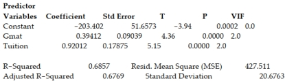Identify the test statistic that should be used to test to determine if the amount of tuition charged by a program is a useful predictor of the average starting salary of the graduates of the program. A) $t = - 3.94$ B) $\mathrm { t } = 4.36$ C) $t = 5.15$ D) $t = 20.67$

Which equation represents a complete second-order model for two quantitative independent variables? A) $E ( y ) = \beta _ { 0 } + \beta _ { 1 } x _ { 1 } + \beta _ { 2 } x _ { 2 } + \beta _ { 3 } x _ { 1 } x _ { 2 } + \beta _ { 4 } x _ { 1 } ^ { 2 } + \beta _ { 5 } x _ { 2 } ^ { 2 }$ B) $E ( y ) = \beta _ { 0 } + \beta _ { 1 } x _ { 1 } + \beta _ { 2 } x _ { 2 } + \beta _ { 3 } x _ { 1 } ^ { 2 } + \beta _ { 4 } x _ { 2 } ^ { 2 }$ C) $E ( y ) = \beta _ { 0 } + \beta _ { 1 } x _ { 1 } x _ { 2 } + \beta _ { 2 } x _ { 1 } ^ { 2 } + \beta _ { 3 } x _ { 2 } ^ { 2 }$ D) $E ( y ) = \beta _ { 0 } + \beta _ { 1 } x _ { 1 } ^ { 2 } + \beta _ { 2 } x _ { 2 } ^ { 2 } + \beta _ { 3 } x _ { 1 } ^ { 2 } x _ { 2 } + \beta _ { 4 } x _ { 1 } x _ { 2 } ^ { 2 } + \beta _ { 5 } x _ { 1 } ^ { 2 } x _ { 2 } ^ { 2 }$

A public health researcher wants to use regression to predict the sun safety knowledge of pre-school children. The researcher randomly sampled 35 preschoolers, assigned them to one of two groups, and then measured the following three variables: SUNSCORE: $\quad y =$ Score on sun-safety comprehension test READING: $\quad \mathrm { x } _ { 1 } =$ Reading comprehension score GROUP: $\quad x _ { 2 } = 1$ if child received a Be Sun Safe demonstration, 0 if not The following two models were hypothesized: Model 1: $E ( y ) = \beta _ { 0 } + \beta _ { 1 } x _ { 1 } + \beta _ { 2 } x _ { 1 } { } ^ { 2 } + \beta _ { 3 } x _ { 2 } + \beta _ { 4 } x _ { 1 } x _ { 2 } + \beta _ { 5 } x _ { 1 } { } ^ { 2 } x _ { 2 }$ Model 2: $\mathrm { E } ( \mathrm { y } ) = \beta _ { 0 } + \beta _ { 1 } \mathrm { x } _ { 1 } + \beta _ { 3 } x _ { 2 } + \beta _ { 4 }x _ { 1 } x _ { 2 }$ A partial f-test was conducted to compare the two models and the resulting p-value was found to be 0.0023. Fill in the blank. The results lead us to conclude that there is (at ? = 0.05).

There are four independent variables, $x _ { 1 } , x _ { 2 } , x _ { 3 }$ , and $x _ { 4 }$ , that might be useful in predicting a response $y$ . A total of $n = 40$ observations is available, and it is decided to employ stepwise regression to help in selecting the independent variables that appear to useful. The computer fits all possible one-variable models of the form $E ( y ) = \beta _ { 0 } + \beta _ { 1 } x _ { i } , i = 1,2,3,4$ . The information in the table is provided from the computer printout. Variable \beta s 1 2.4 0.52 2 -0.2 0.03 3 3.6 2.11 4 0.8 0.44 Which independent variable is declared the best one-variable predictor of $y$ ? A) $x _ { 1 }$ B) $x_ 2$ C) $x _ { 3 }$ D) $x _ { 4 }$

Probabilistic models that include more than one dependent variable are called multiple regression models.

As part of a study at a large university, data were collected on n = 224 freshmen computer science (CS) majors in a particular year. The researchers were interested in modeling y, a student's grade point average (GPA) after three semesters, as a function of the following independent variables (recorded at the time the students enrolled in the university): $x _ { 1 } =$ average high school grade in mathematics (HSM) $x _ { 2 } =$ average high school grade in science (HSS) $x _ { 3 } =$ average high school grade in English (HSE) $x _ { 4 } =$ SAT mathematics score (SATM) $x _ { 5 } =$ SAT verbal score (SATV) A first-order model was fit to data. A $95 \%$ confidence interval for $\beta _ { 1 }$ is $( .06 , .22 )$ . Interpret this result. A) We are $95 \%$ confident that a CS freshman's GPA increases by an amount between .06 and .22 for every 1 -point increase in average H5 math grade, holding $x _ { 2 } - x _ { 5 }$ constant. B) $95 \%$ of the GPAs fall within .06 to $.22$ of their true values. C) We are $95 \%$ confident that a CS freshman's HS math grade increases by an amount between .06 and .22 for every 1-point increase in GPA, holding $x _ { 2 } - x _ { 5 }$ constant. D) We are $95 \%$ confident that the mean GPA of all CS freshmen after three semesters falls between .06 and $.22$ .

In situations where two competing models have essentially the same predictive power (as determined by an F-test), it is standard procedure to use the model with the greater number of parameters.

The table shows the profit y (in thousands of dollars) that a company made during a month when the price of its product was x dollars per unit. Profit, y Price, x 12 1.20 17 1.25 20 1.29 21 1.30 24 1.35 26 1.39 27 1.40 23 1.45 21 1.49 20 1.50 15 1.55 11 1.59 10 1.60 5 1.65 a. Fit the model $y = \beta _ { 0 } + \beta _ { 1 } x + \beta _ { 2 } x 2 + \varepsilon$ to the data and give the least squares prediction equation. b. Plot the fitted equation on a scattergram of the data. c. Is there sufficient evidence of downward curvature in the relationship between profit and price? Use $\alpha = .05$ . 4 Perform Quadratic Regression and Make Predictions

The model $E ( y ) = \beta _ { 0 } + \beta _ { 1 } x _ { 1 } + \beta _ { 2 } x _ { 2 }$ was fit to a set of data. A partial printout for the analysis follows: Actual Predict Lower 95\% CL Upper 95\% CL OBS 1 2 Value Value Residual Predict Predict 1 7781 644 74.707 83.175 -8.468 47.224 119.126 Interpret the value of the residual when $x _ { 1 } = 7,781$ and $x _ { 2 } = 644$ . A) The predicted $\hat{y}$ exceeds the observed value of $y$ by $8.468$ . B) The predicted $\hat{y}$ is $8.468$ less than the observed value of $y$ . C) Since the residual is negative, there is evidence of a negative linear relationship between $y$ and at least one of the two independent variables. D) Since the residual is not 0 , the model is not useful for predicting $y$ .

A public health researcher wants to use regression to predict the sun safety knowledge of pre-school children. The researcher randomly sampled 35 preschoolers, assigned them to one of two groups, and then measured the following three variables: SUNSCORE: $\quad \mathrm { y } =$ Score on sun-safety comprehension test READING: $\quad \mathrm { x } _ { 1 } =$ Reading comprehension score GROUP: $\quad x _ { 2 } = 1$ if child received a Be Sun Safe demonstration, 0 if not A regression model was fit and the following residual plot was observed. 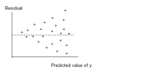Which of the following assumptions appears violated based on this plot?

As part of a study at a large university, data were collected on n = 224 freshmen computer science (CS) majors in a particular year. The researchers were interested in modeling y, a student's grade point average (GPA) after three semesters, as a function of the following independent variables (recorded at the time the students enrolled in the university): $x _ { 1 } =$ average high school grade in mathematics (HSM) $x _ { 2 } =$ average high school grade in science (HSS) $x _ { 3 } =$ average high school grade in English (HSE) $x _ { 4 } =$ SAT mathematics score (SATM) $x _ { 5 } =$ SAT verbal score (SATV) A first-order model was fit to data with $R _ { a } ^ { 2 } = .193$ . Interpret the value of the adjusted coefficient of determination $R _ { a } ^ { 2 }$ .

The first-order model below was fit to a set of data. $E ( y ) = \beta _ { 0 } + \beta _ { 1 } x _ { 1 } + \beta _ { 2 } x _ { 2 }$ Explain how to determine if the constant variance assumption is satisfied.

We decide to conduct a multiple regression analysis to predict the attendance at a major league baseball game. We use the size of the stadium as a quantitative independent variable and the type of game as a qualitative variable (with two levels - day game or night game). We hypothesize the following model: $E ( y ) = \beta _ { 0 } + \beta _ { 1 } x _ { 1 } + \beta _ { 2 } x _ { 2 } + \beta _ { 3 } x _ { 3 }$ Where $\mathrm { x } _ { 1 } =$ size of the stadium $\mathrm { x } _ { 2 } = 1$ if a day game, 0 if a night game A plot of the $y - x _ { 1 }$ relationship would show: :

Twenty colleges each recommended one of its graduating seniors for a prestigious graduate fellowship. The process to determine which student will receive the fellowship includes several interviews. The gender of each student and his or her score on the first interview are shown below. Student Gender Score 1 Male 18 2 Female 17 3 Female 19 4 Female 16 5 Male 12 6 Female 15 7 Female 18 8 Male 16 9 Male 18 10 Female 20 Student Gender Score 11 Female 17 12 Male 16 13 Male 16 14 Female 19 15 Female 16 16 Male 15 17 Female 12 18 Male 14 19 Female 16 20 Female 18 a. Suppose you want to use gender to model the score on the interview y. Create the appropriate number of dummy variables for gender and write the model. b. Fit the model to the data. c. Give the null hypothesis for testing whether gender is a useful predictor of the score y. d. Conduct the test and give the appropriate conclusion. Use α = .05. 12.8 Models with Both Quantitative and Qualitative Variables (Optional) 1 Write and Interpret Model with Quantitative and Qualitative Variables

The model $E ( y ) = \beta _ { 0 } + \beta _ { 1 } x$ was fit to a set of data, and the following plot of residuals against x values was obtained. 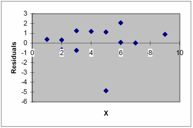Interpret the residual plot. 12.12 Some Pitfalls: Estimability, Multicollinearity, and Extrapolation

A study of the top MBA programs attempted to predict the average starting salary (in $1000's) of graduates of the program based on the amount of tuition (in $1000's) charged by the program and the average GMAT score of the program's students. The results of a regression analysis based on a sample of 75 MBA programs is shown below: Least Squares Linear Regression of Salary 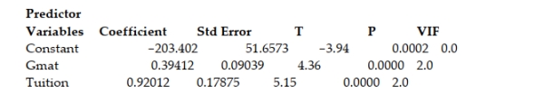The model was then used to create 95% confidence and prediction intervals for y and for E(Y) when the tuition charged by the MBA program was $75,000 and the GMAT score was 675. The results are shown here: 95% confidence interval for E(Y): ($126,610, $136,640) 95% prediction interval for Y: ($90,113, $173,160) Which of the following interpretations is correct if you want to use the model to estimate E(Y) for all MBA programs?

Consider the model $y = \beta _ { 0 } + \beta _ { 1 } x _ { 1 } + \beta _ { 2 } x _ { 2 } + \beta _ { 3 } x _ { 3 } + \varepsilon$ where $x _ { 1 }$ is a quantitative variable and $x _ { 2 }$ and $x _ { 3 }$ are dummy variables describing a qualitative variable at three levels using the coding scheme $x _ { 2 } = \left\{ \begin{array} { l l } 1 & \text { if level 2 } \\0 & \text { otherwise }\end{array} \quad x _ { 3 } = \left\{ \begin{array} { l l } 1 & \text { if level 3 } \\0 & \text { otherwise }\end{array} \right. \right.$ The resulting least squares prediction equation is $\hat { y } = 36.7 + 1.3 x _ { 1 } + 5.4 x _ { 2 } + 3.2 x _ { 3 }$ . What is the least squares regression equation associated with level 2? A) $\hat { y } = 42.1 + 1.3 x _ { 1 }$ B) $\hat { y }= 39.9 + 1.3 x _ { 1 }$ C) $\hat { y } = 38.0 + 5.4 x _ { 2 }$ D) $\hat { y } = 39.9 + 5.4 x _ { 2 }$

Consider the interaction model $E ( y ) = 3.6 + 1.2 x _ { 1 } + 2.4 x _ { 2 } + .2 x _ { 1 } x _ { 2 }$ . Determine the change in $E ( y )$ when $x _ { 1 }$ is changed from 6 to 7 and $x _ { 2 }$ is held fixed at 3 . A) $1.8$ B) $10.8$ C) $11.4$ D) $4.2$