Question 1

A polynomial regression model is specified as:

Accepted Answer

A) Yi = ?0 + ?1Xi + ?2X $\begin{array} { l } 
2 \
i
\end{array}$ + ??? + ?rX $\begin{array} { l } 
r\
i
\end{array}$ + ui. 
B) Yi = ?0 + ?1Xi + ? $\begin{array} { l } 
2 \
1
\end{array}$ Xi + ??? + ? $\begin{array} { l } 
r \
1
\end{array}$ Xi + ui. 
C) Yi = ?0 + ?1Xi + ?2Y $\begin{array} { l } 
2 \
i
\end{array}$ + ??? + ?rY $\begin{array} { l } 
r \
i
\end{array}$ + ui. 
D) Yi = ?0 + ?1X1i + ?2X2 + ?3 (X1i × X2i)+ ui. 
A) Yi = ?0 + ?1Xi + ?2X $\begin{array} { l } 
2 \
i
\end{array}$ + ??? + ?rX $\begin{array} { l } 
r\
i
\end{array}$ + ui. 
B) Yi = ?0 + ?1Xi + ? $\begin{array} { l } 
2 \
1
\end{array}$ Xi + ??? + ? $\begin{array} { l } 
r \
1
\end{array}$ Xi + ui. 
C) Yi = ?0 + ?1Xi + ?2Y $\begin{array} { l } 
2 \
i
\end{array}$ + ??? + ?rY $\begin{array} { l } 
r \
i
\end{array}$ + ui. 
D) Yi = ?0 + ?1X1i + ?2X2 + ?3 (X1i × X2i)+ ui.

Question 2

To test whether or not the population regression function is linear rather than a polynomial of order r,

Accepted Answer

A) check whether the regression R2 for the polynomial regression is higher than that of the linear regression. 
B) compare the TSS from both regressions. 
C) look at the pattern of the coefficients: if they change from positive to negative to positive, etc., then the polynomial regression should be used. 
D) use the test of (r-1)restrictions using the F-statistic. 
A) check whether the regression R2 for the polynomial regression is higher than that of the linear regression. 
B) compare the TSS from both regressions. 
C) look at the pattern of the coefficients: if they change from positive to negative to positive, etc., then the polynomial regression should be used. 
D) use the test of (r-1)restrictions using the F-statistic.

Question 3

The figure shows is a plot and a fitted linear regression line of the age-earnings profile of 1,744 individuals, taken from the Current Population Survey. 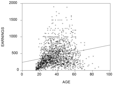  (a)Describe the problems in predicting earnings using the fitted line. What would the pattern of the residuals look like for the age category under 40?
(b)What alternative functional form might fit the data better?
(c)What other variables might you want to consider in specifying the determinants of earnings?

Accepted Answer

(a)There would be many overpredictions f

Question 4

The interpretation of the slope coefficient in the model Yi = β0 + β1 ln(Xi)+ ui is as follows:

Accepted Answer

A) a 1% change in X is associated with a β1 % change in Y. 
B) a 1% change in X is associated with a change in Y of 0.01 β1. 
C) a change in X by one unit is associated with a β1 100% change in Y. 
D) a change in X by one unit is associated with a β1 change in Y. 
A) a 1% change in X is associated with a β1 % change in Y. 
B) a 1% change in X is associated with a change in Y of 0.01 β1. 
C) a change in X by one unit is associated with a β1 100% change in Y. 
D) a change in X by one unit is associated with a β1 change in Y.

Question 5

In the model Yi = ?0 + ?1X1 + ?2X2 + ?3(X1 × X2)+ ui, the expected effect $\frac { \Delta Y } { \Delta X _ { 1 } }$ is

Accepted Answer

A) ?1 + ?3X2. 
B) ?1. 
C) ?1 + ?3. 
D) ?1 + ?3X1. 
A) ?1 + ?3X2. 
B) ?1. 
C) ?1 + ?3. 
D) ?1 + ?3X1.

Question 6

The following interactions between binary and continuous variables are possible, with the exception of

Accepted Answer

A) Yi = β0 + β1Xi + β2Di + β3(Xi × Di)+ ui. 
B) Yi = β0 + β1Xi + β2(Xi × Di)+ ui. 
C) Yi = (β0 + Di)+ β1Xi + ui. 
D) Yi = β0 + β1Xi + β2Di + ui. 
A) Yi = β0 + β1Xi + β2Di + β3(Xi × Di)+ ui. 
B) Yi = β0 + β1Xi + β2(Xi × Di)+ ui. 
C) Yi = (β0 + Di)+ β1Xi + ui. 
D) Yi = β0 + β1Xi + β2Di + ui.

Question 7

Table 8.1 on page 284 of your textbook displays the following estimated earnings function in column (4): $$\begin{aligned}
\widehat { T \text { eamings } } = & 1.503 + 0.1032 \times \text { educ } - 0.451 \times \text { DFemme } + 0.0143 \times ( \text { DFemme } \times \text { educ } ) \
& ( 0.023 ) ( 0.0012 ) \quad \quad\quad\quad( 0.024 )\quad\quad\quad\quad\quad( 0.0017 )
\end{aligned}$$

$$\begin{array} { c c c c c } 
+ 0.0232 \times \text { exper } - 0.000368 \times \text { exper } 2 - 0.058 \times \text { Midwest } - 0.0098 \times \text { South } - 0.030 \times \text { West } \
( 0.0012 ) \quad\quad\quad ( 0.000023 ) \quad\quad\quad ( 0.006 ) \quad\quad\quad\quad ( 0.006 ) \quad\quad\quad\quad\quad ( 0.007 )
\end{array}$$

$$n = 52.790 , \overline { \mathrm { R } } ^ { 2 } = 0.267$$
Given that the potential experience variable (exper)is defined as (Age-Education-6)find the age at which individuals with a high school degree (12 years of education)and with a college degree (16 years of education)have maximum earnings, holding all other factors constant.

Accepted Answer

The earnings function is a quadratic fun

Question 8

(Requires Calculus)In the equation $\widehat{\text { TestScore }}$ = 607.3 + 3.85 Income - 0.0423Income2, the following income level results in the maximum test score

Accepted Answer

A) 607.3. 
B) 91.02. 
C) 45.50. 
D) cannot be determined without a plot of the data. 
A) 607.3. 
B) 91.02. 
C) 45.50. 
D) cannot be determined without a plot of the data.

Question 9

Many countries that experience hyperinflation do not have market-determined interest rates. As a result, some authors have substituted future inflation rates into money demand equations of the following type as a proxy: $m = \beta _ { 0 } \times ( 1 + \Delta \ln P ) ^ { \beta _ { 1 } } \times e ^ { u }$ (m is real money, and P is the consumer price index).
Income is typically omitted since movements in it are dwarfed by money growth and the inflation rate. Authors have then interpreted β1 as the "semi-elasticity" of the inflation rate. Do you see any problems with this interpretation?

Accepted Answer

Linearizing the above equation results i

Question 10

In the regression model Yi = β0 + β1Xi + β2Di + β3(Xi × Di)+ ui, where X is a continuous variable and D is a binary variable, β2

Accepted Answer

A) is the difference in means in Y between the two categories. 
B) indicates the difference in the intercepts of the two regressions. 
C) is usually positive. 
D) indicates the difference in the slopes of the two regressions. 
A) is the difference in means in Y between the two categories. 
B) indicates the difference in the intercepts of the two regressions. 
C) is usually positive. 
D) indicates the difference in the slopes of the two regressions.

Question 11

To decide whether Yi = β0 + β1X + ui or ln(Yi)= β0 + β1X + ui fits the data better, you cannot consult the regression R2 because

Accepted Answer

A) ln(Y)may be negative for 0<Y<1. 
B) the TSS are not measured in the same units between the two models. 
C) the slope no longer indicates the effect of a unit change of X on Y in the log-linear model. 
D) the regression R2 can be greater than one in the second model. 
A) ln(Y)may be negative for 0<Y<1. 
B) the TSS are not measured in the same units between the two models. 
C) the slope no longer indicates the effect of a unit change of X on Y in the log-linear model. 
D) the regression R2 can be greater than one in the second model.

Question 12

In estimating the original relationship between money wage growth and the unemployment rate, Phillips used United Kingdom data from 1861 to 1913 to fit a curve of the following functional form
( $\frac { \dot { W } } { W }$ + β0)= β1 × $ur \beta _ { 2 }$ × eu,
where $\frac { \dot { W } } { W }$ is the percentage change in money wages and ur is the unemployment rate. Sketch the function. What role does β0 play? Can you find a linear transformation that allows you to estimate the above function using OLS? If, after taking logarithms on both sides of the equation, you tried to estimate β1 and β2 using OLS by choosing different values for β0 by "trial and error procedure" (Phillips's words), what sort of problem might you run into with the left-hand side variable for some of the observations?

Accepted Answer

Given the shape of the Phillips curve, β

Question 13

Give at least three examples from economics where you expect some nonlinearity in the relationship between variables. Interpret the slope in each case.

Accepted Answer

Answers will vary by student.

Question 14

A nonlinear function

Accepted Answer

A) makes little sense, because variables in the real world are related linearly. 
B) can be adequately described by a straight line between the dependent variable and one of the explanatory variables. 
C) is a concept that only applies to the case of a single or two explanatory variables since you cannot draw a line in four dimensions. 
D) is a function with a slope that is not constant. 
A) makes little sense, because variables in the real world are related linearly. 
B) can be adequately described by a straight line between the dependent variable and one of the explanatory variables. 
C) is a concept that only applies to the case of a single or two explanatory variables since you cannot draw a line in four dimensions. 
D) is a function with a slope that is not constant.

Question 15

One of the most frequently estimated equations in the macroeconomics growth literature are so-called convergence regressions. In essence the average per capita income growth rate is regressed on the beginning-of-period per capita income level to see if countries that were further behind initially, grew faster. Some macroeconomic models make this prediction, once other variables are controlled for. To investigate this matter, you collect data from 104 countries for the sample period 1960-1990 and estimate the following relationship (numbers in parentheses are for heteroskedasticity-robust standard errors): $\begin{aligned}
\widehat { g 6090 } = & 0.020 - 0.360 \times \text { gpop } + 0.004 \times \text { Educ } - 0.053 \times \text { RelProd } _ { 60 } , R ^ { 2 } = 0.332 , \text { SER } = 0.013 \
& ( 0.009 ) ( 0.241 )\quad \quad\quad \quad(0.001)\quad \quad\quad \quad(0.009)
\end{aligned}$
where g6090 is the growth rate of GDP per worker for the 1960-1990 sample period, RelProd60 is the initial starting level of GDP per worker relative to the United States in 1960, gpop is the average population growth rate of the country, and Educ is educational attainment in years for 1985.
(a)What is the effect of an increase of 5 years in educational attainment? What would happen if a country could implement policies to cut population growth by one percent? Are all coefficients significant at the 5% level? If one of the coefficients is not significant, should you automatically eliminate its variable from the list of explanatory variables?
(b)The coefficient on the initial condition has to be significantly negative to suggest conditional convergence. Furthermore, the larger this coefficient, in absolute terms, the faster the convergence will take place. It has been suggested to you to interact education with the initial condition to test for additional effects of education on growth. To test for this possibility, you estimate the following regression: $\begin{array} { l } 
\widehat { g 6090 } = 0.015 - 0.323 \times \text { gpop } + 0.005 \times \text { Educ } - 0.051 \times \text { RelProd } _ { 60 } \
\quad \quad\quad \quad( 0.009 ) ( 0.238 )\quad \quad \quad ( 0.001 ) \quad \quad\quad \quad( 0.013 ) \\
- 0.0028 \times ( \text { EducRelProd } 60 ) , R ^ { 2 } = 0.346 , \mathrm { SER } = 0.013 \
( 0.0015 )
\end{array}$
Write down the effect of an additional year of education on growth. West Germany has a value for RelProd60 of 0.57, while Brazil's value is 0.23. What is the predicted growth rate effect of adding one year of education in both countries? Does this predicted growth rate make sense?
(c)What is the implication for the speed of convergence? Is the interaction effect statistically significant?
(d)Convergence regressions are basically of the type
?ln Yt = ?0 - ?1 ln Y0
where ? might be the change over a longer time period, 30 years, say, and the average growth rate is used on the left-hand side. You note that the equation can be rewritten as
?ln Yt = ?0 - (1 - ?1)ln Y0
Over a century ago, Sir Francis Galton first coined the term "regression" by analyzing the relationship between the height of children and the height of their parents. Estimating a function of the type above, he found a positive intercept and a slope between zero and one. He therefore concluded that heights would revert to the mean. Since ultimately this would imply the height of the population being the same, his result has become known as "Galton's Fallacy." Your estimate of ?1 above is approximately 0.05. Do you see a parallel to Galton's Fallacy?

Accepted Answer

(a)Increasing educational attainment by

Question 16

The exponential function

Accepted Answer

A) is the inverse of the natural logarithm function. 
B) does not play an important role in modeling nonlinear regression functions in econometrics. 
C) can be written as exp(ex). 
D) is ex, where e is 3.1415…. 
A) is the inverse of the natural logarithm function. 
B) does not play an important role in modeling nonlinear regression functions in econometrics. 
C) can be written as exp(ex). 
D) is ex, where e is 3.1415….

Question 17

Earnings functions attempt to predict the log of earnings from a set of explanatory variables, both binary and continuous. You have allowed for an interaction between two continuous variables: education and tenure with the current employer. Your estimated equation is of the following type: $\widehat{\text { In Earn }}$ = $\hat { \beta }$ 0 + $\hat { \beta }$ 1 × Femme + $\hat { \beta }$ 2 × Educ + $\hat { \beta }$ 3 × Tenure + $\hat { \beta }$ 4 x (Educ × Tenure)+ ∙∙∙
where Femme is a binary variable taking on the value of one for females and is zero otherwise, Educ is the number of years of education, and tenure is continuous years of work with the current employer. What is the effect of an additional year of education on earnings ("returns to education")for men? For women? If you allowed for the returns to education to differ for males and females, how would you respecify the above equation? What is the effect of an additional year of tenure with a current employer on earnings?

Accepted Answer

For both males and females, the effect o

Question 18

An example of a quadratic regression model is

Accepted Answer

A) Yi = ?0 + ?1X + ?2Y2 + ui. 
B) Yi = ?0 + ?1ln(X)+ ui. 
C) Yi = ?0 + ?1X + ?2X2 + ui. 
D)  $Y _ { i } ^ { 2 }$ = ?0 + ?1X + ui. 
A) Yi = ?0 + ?1X + ?2Y2 + ui. 
B) Yi = ?0 + ?1ln(X)+ ui. 
C) Yi = ?0 + ?1X + ?2X2 + ui. 
D)  $Y _ { i } ^ { 2 }$ = ?0 + ?1X + ui.

Question 19

Earnings functions attempt to find the determinants of earnings, using both continuous and binary variables. One of the central questions analyzed in this relationship is the returns to education.
(a)Collecting data from 253 individuals, you estimate the following relationship 
$\begin{array} { c } 
\widehat { \ln \left( \text { Eam } _ { i } \right) }= 0.54 + 0.083 \times E d u c ,  R ^ { 2 } = 0.20 , S E R = 0.445 \
( 0.14 ) ( 0.011 )
\end{array}$
where Earn is average hourly earnings and Educ is years of education.
What is the effect of an additional year of schooling? If you had a strong belief that years of high school education were different from college education, how would you modify the equation? What if your theory suggested that there was a "diploma effect"?
(b)You read in the literature that there should also be returns to on-the-job training. To approximate on-the-job training, researchers often use the so called Mincer or potential experience variable, which is defined as Exper = Age - Educ - 6. Explain the reasoning behind this approximation. Is it likely to resemble years of employment for various sub-groups of the labor force?
(c)You incorporate the experience variable into your original regression $\begin{array} { r } 
\widehat{ { ln(\text {Earn}_{i})} } = - 0.01 + 0.101 \times \text { Educ } + 0.033 \times \text { Exper } - 0.0005 \times \text { Exper } 2 \
\end{array}$
$\quad $$\quad $$\quad $$\quad $$\quad $$\quad $( 0.16 ) ( 0.012 )$\quad $$\quad $$\quad $$\quad $$\quad $$\quad $$\quad $$\quad $$\quad $(0.006)$\quad $$\quad $$\quad $$\quad $$\quad $$\quad $(0.0001)
$$R ^ { 2 } = 0.34 , S E R = 0.405$$
What is the effect of an additional year of experience for a person who is 40 years old and had 12 years of education? What about for a person who is 60 years old with the same education background?
(d)Test for the significance of each of the coefficients of the added variables. Why has the coefficient on education changed so little? Sketch the age-(log)earnings profile for workers with 8 years of education and 16 years of education.
(e)You want to find the effect of introducing two variables, gender and marital status. Accordingly you specify a binary variable that takes on the value of one for females and is zero otherwise (Female), and another binary variable that is one if the worker is married but is zero otherwise (Married). Adding these variables to the regressors results in: $\begin{array}{l}
\begin{array} { l } 
\widehat { \ln \left( \text { Earn } _ { i } \right) } = 0.21 + 0.093 \times \text { Educ } + 0.032 \times \text { Exper } - 0.0005 \times \text { Exper } ^ { 2 } \
\quad \quad \quad \quad \quad \text { (0.16) } ( 0.012 ) \quad\quad \quad \quad  ( 0.006 ) \quad\quad \quad \quad \quad  ( 0.0001 ) \
- 0.289 \times \text { Female } + 0.062 \text { Married, } \
\text { (0.049) \quad \quad \quad \quad \quad (0.056) } \
\end{array}\\
R ^ { 2 } = 0.43 , S E R = 0.378
\end{array}$
Are the coefficients of the two added binary variables individually statistically significant? Are they economically important? In percentage terms, how much less do females earn per hour, controlling for education and experience? How much more do married people make? What is the percentage difference in earnings between a single male and a married female? What is the marriage differential between males and females?
(f)In your final specification, you allow for the binary variables to interact. The results are as follows: $$\begin{array} { l } 
\widehat { \ln \left( \text { Earn } _ { i } \right) } = 0.14 + 0.093 \times \text { Educ } + 0.032 \times \text { Exper } - 0.0005 \times \text { Exper } 2 \
\quad \quad \quad \quad \quad \text { (0.16) } ( 0.011 ) \quad \quad \quad \quad ( 0.006 ) \quad \quad \quad \quad \quad ( 0.001 ) \
- 0.158 \times \text { Female } + 0.173 \times \text { Married } - 0.218 \times ( \text { Female } \times \text { Married } ) \text {, } \
\text { (0.075) }\quad \quad\quad \quad\quad \quad ( 0.080 )\quad \quad\quad \quad(0.097)\
\end{array}$$

$$R ^ { 2 } = 0.44 , S E R = 0.375$$
Repeat the exercise in (e)of calculating the various percentage differences between gender and marital status.

Accepted Answer

(a)One additional year of education carr

Question 20

In the case of perfect multicollinearity, OLS is unable to estimate the slope coefficients of the variables involved. Assume that you have included both X1 and X2 as explanatory variables, and that X2 = X $\begin{array} { l } 
2 \
1
\end{array}$ , so that there is an exact relationship between two explanatory variables. Does this pose a problem for estimation?

Accepted Answer

There is no problem for estimation, sinc

A polynomial regression model is specified as:

To test whether or not the population regression function is linear rather than a polynomial of order r,

The interpretation of the slope coefficient in the model Y_i = β₀ + β₁ ln(X_i)+ u_i is as follows:

In the model Y_i = ?₀ + ?₁X₁+ ?₂X₂ + ?₃(X₁ × X₂)+ u_i, the expected effect $\frac { \Delta Y } { \Delta X _ { 1 } }$ is

The following interactions between binary and continuous variables are possible, with the exception of

(Requires Calculus)In the equation $\widehat{\text { TestScore }}$ = 607.3 + 3.85 Income - 0.0423Income², the following income level results in the maximum test score

In the regression model Y_i = β₀ + β₁X_i+ β₂D_i + β₃(X_i × D_i)+ u_i, where X is a continuous variable and D is a binary variable, β₂

To decide whether Y_i = β₀ + β₁X + u_i or ln(Y_i)= β₀ + β₁X + u_i fits the data better, you cannot consult the regression R² because

Give at least three examples from economics where you expect some nonlinearity in the relationship between variables. Interpret the slope in each case.

A nonlinear function

The exponential function

An example of a quadratic regression model is

Economic Questions and Data

Review of Probability

Review of Statistics

Linear Regression With One Regressor

Regression With a Single Regressor: Hypothesis Tests and Confidence Intervals

Linear Regression With Multiple Regressors

Hypothesis Tests and Confidence Intervals in Multiple Regression

Assessing Studies Based on Multiple Regression

Regression With Panel Data

Regression With a Binary Dependent Variable

Instrumental Variables Regression

Experiments and Quasi-Experiments

Introduction to Time Series Regression and Forecasting

Estimation of Dynamic Causal Effects

Additional Topics in Time Series Regression

The Theory of Linear Regression With One Regressor

The Theory of Multiple Regression

Filters

Exam 8: Nonlinear Regression Functions

A polynomial regression model is specified as:

To test whether or not the population regression function is linear rather than a polynomial of order r,

The interpretation of the slope coefficient in the model Yi = β0 + β1 ln(Xi)+ ui is as follows:

In the model Yi = ?0 + ?1X1 + ?2X2 + ?3(X1 × X2)+ ui, the expected effect ΔYΔX1\frac { \Delta Y } { \Delta X _ { 1 } }ΔX1​ΔY​ is

The following interactions between binary and continuous variables are possible, with the exception of

(Requires Calculus)In the equation TestScore ^\widehat{\text { TestScore }} TestScore = 607.3 + 3.85 Income - 0.0423Income2, the following income level results in the maximum test score

In the regression model Yi = β0 + β1Xi + β2Di + β3(Xi × Di)+ ui, where X is a continuous variable and D is a binary variable, β2

To decide whether Yi = β0 + β1X + ui or ln(Yi)= β0 + β1X + ui fits the data better, you cannot consult the regression R2 because

Give at least three examples from economics where you expect some nonlinearity in the relationship between variables. Interpret the slope in each case.

A nonlinear function

The exponential function

An example of a quadratic regression model is

Economic Questions and Data

Review of Probability

Review of Statistics

Linear Regression With One Regressor

Regression With a Single Regressor: Hypothesis Tests and Confidence Intervals

Linear Regression With Multiple Regressors

Hypothesis Tests and Confidence Intervals in Multiple Regression

Assessing Studies Based on Multiple Regression

Regression With Panel Data

Regression With a Binary Dependent Variable

Instrumental Variables Regression

Experiments and Quasi-Experiments

Introduction to Time Series Regression and Forecasting

Estimation of Dynamic Causal Effects

Additional Topics in Time Series Regression

The Theory of Linear Regression With One Regressor

The Theory of Multiple Regression

Filters

The interpretation of the slope coefficient in the model Y_i = β₀ + β₁ ln(X_i)+ u_i is as follows:

In the model Y_i = ?₀ + ?₁X₁+ ?₂X₂ + ?₃(X₁ × X₂)+ u_i, the expected effect $\frac { \Delta Y } { \Delta X _ { 1 } }$ is

(Requires Calculus)In the equation $\widehat{\text { TestScore }}$ = 607.3 + 3.85 Income - 0.0423Income², the following income level results in the maximum test score

In the regression model Y_i = β₀ + β₁X_i+ β₂D_i + β₃(X_i × D_i)+ u_i, where X is a continuous variable and D is a binary variable, β₂

To decide whether Y_i = β₀ + β₁X + u_i or ln(Y_i)= β₀ + β₁X + u_i fits the data better, you cannot consult the regression R² because