Exam 9: Assessing Studies Based on Multiple Regression

Sir Francis Galton (1822-1911), an anthropologist and cousin of Charles Darwin, created the term regression. In his article "Regression towards Mediocrity in Hereditary Stature," Galton compared the height of children to that of their parents, using a sample of 930 adult children and 205 couples. In essence he found that tall (short)parents will have tall (short)offspring, but that the children will not be quite as tall (short)as their parents, on average. Hence there is regression towards the mean, or as Galton referred to it, mediocrity. This result is obviously a fallacy if you attempted to infer behavior over time since, if true, the variance of height in humans would shrink over generations. This is not the case. (a)To research this result, you collect data from 110 college students and estimate the following relationship: $\widehat { \text { studenth } } = 19.6 + 0.73 \times \text { Midparh, } R ^ { 2 } = 0.45 , S E R = 2.0$ $\quad$$\quad$$\quad$$\quad$$\quad$ (7.2) $( 0.10 )$ where Studenth is the height of students in inches and Midparh is the average of the parental heights. Values in parentheses are heteroskedasticity-robust standard errors. Sketching this regression line together with the 45 degree line, explain why the above results suggest "regression to the mean" or "mean reversion." (b)Researching the medical literature, you find that height depends, to a large extent, on one gene ("phog")and on environmental influences. Let us assume that parents and offspring have the same invariant (over time)gene and that actual height is therefore measured with error in the following sense, $\tilde { X _ { i , 0 } } = X _ { i } + v _ { i , 0 } \text { and } \tilde { X _ { i , p } } = X _ { i } + w _ { i , p }$ where $\bar { X }$ is measured height, X is the height given through the gene, v and w are environmental influences, and the subscripts o and p stand for offspring and parents, respectively. Let the environmental influences be independent from each other and from the gene. Subtracting the measured height of offspring from the height of parents, what sort of population regression function do you expect? (c)How would you test for the two restrictions implicit in the population regression function in (b)? Can you tell from the results in (a)whether or not the restrictions hold? (d)Proceeding in a similar way to the proof in your textbook, you can show that $\hat { \beta } _ { 1 }\xrightarrow{p} 1 - \frac { \sigma _ { v } ^ { 2 } } { \sigma _ { X } ^ { 2 } + \sigma _ { v } ^ { 2 } }$ for the situation in (b). Discuss under what conditions you will find a slope closer to one for the height comparison. Under what conditions will you find a slope closer to zero? (e)Can you think of other examples where Galton's Fallacy might apply?

By including another variable in the regression, you will

Keynes postulated that the marginal propensity to consume (MPC = $\frac { \Delta C } { \Delta Y _ { p d } }$ )is between zero and one. He also hypothesized that the average propensity to consume (APC = $\frac { \Delta C } { \Delta Y _ { p d } }$ )would fall as personal disposable income $Y _ { p d }$ increased. (a)Specify a linear consumption function. Show that the assumption of a falling APC implies the presence of a positive intercept. (b)Using annual per capita data, estimation of the consumption function for the United States results in the following output for the years 1929-1938: $\hat { C } _ { t }$ = 981.35 + 0.735 $Y _ { p d , t }$ , R² = 0.98, SER= 50.65 (158.65)(0.038) Can you reject the null hypothesis that the slope is less than one? Greater than zero? Test the hypothesis that the intercept is zero. Should you be concerned about the sample size when conducting these tests? What other threats to internal validity may be present here? (c)Given the GDP identity for a closed economy, $Y _ { t } \equiv C _ { t } + I _ { t } + G _ { t }$ show why economists saw important policy implications in finding an APC that would decrease over time. (d)Simon Kuznets, who won the Nobel Prize in economics, collected data on consumption expenditures and national income from 1869 to 1938 and found, using overlapping period averages, that the APC was relatively constant over this period. To reconcile this finding with the regression results, Milton Friedman, who also won the Nobel Prize, formulated the "permanent income" hypothesis. In essence, Friedman hypothesized that both actual consumption and income are measured with error, $\overline { C _ { t } } = C _ { t } + v _ { t }$ and $\bar { Y } _ { t } = Y _ { t } + w _ { s }$ where $C _ { t }$ and $Y _ { t }$ were called "permanent" consumption and income, respectively, and $v _ { t }$ and $w _ { t }$ , the two measurement errors, were labeled transitory consumption and income. Friedman hypothesized that the transitory components were purely random error terms, uncorrelated with the permanent parts. Let permanent consumption and income be related as follows: $C _ { t } = k \times Y _ { p d t } + u _ { t }$ so that the APC and MPC are the same and constant over time. Furthermore, let both transitory and permanent income be independent of the error term. Show that by regressing actual consumption on actual income, the MPC will be downward biased, and the intercept will be greater than zero, even in large samples (to simplify the analysis, assume that permanent income and all of the errors are i.i.d. and mutually independent).

Your textbook uses the following example of simultaneous causality bias of a two equation system: Y_i = β₀ + β₁X_i + u_i X_i = $\gamma _ { 0 }$ + $\gamma _ { 1 }$ Y_i + v_i To be more specific, think of the first equation as a demand equation for a certain good, where Y is the quantity demanded and X is the price. The second equation then represents the supply equation, with a third equation establishing that demand equals supply. Sketch the market outcome over a few periods and explain why it is impossible to identify the demand and supply curves in such a situation. Next assume that an additional variable enters the demand equation: income. In a new graph, draw the initial position of the demand and supply curves and label them D⁰ and S⁰. Now allow for income to take on four different values and sketch what happens to the two curves. Is there a pattern that you see which suggests that you might be able to identify one of the two equations with real-life data?

Correlation of the regression error across observations

Several authors have tried to measure the "persistence" in U.S state unemployment rates by running the following regression: $u r _ { i , t } = \beta _ { 0 } + \beta _ { 1 } \times u r _ { i , t - k } + z _ { i , t }$ where ur is the state unemployment rate, i is the index for the i-th state, t indicates a time period, and typically k ? 10. (a)Explain why finding a slope estimate of one and an intercept of zero is typically interpreted as evidence of "persistence." (b)You collect data on the 48 contiguous U.S. states' unemployment rates and find the following estimates: $\hat { u } r _ { i , 1995 }$ = 2.25 + 0.60 × $u r _ { i , 1970 }$ ; R² = 0.40, SER = 0.90 (0.61)(0.13) Interpret the regression results. (c)Analyzing the accompanying figure, and interpret the observation for Maryland and for Washington. Do you find evidence of persistence? How would you test for it? 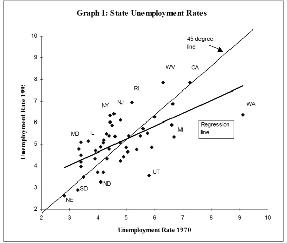(d)One of your peers points out that this result makes little sense, since it implies that eventually all states would have identical unemployment rates. Explain the argument. (e)Imagine that state unemployment rates were determined by their natural rates and some transitory shock. The natural rates themselves may be functions of the unemployment insurance benefits of the state, unionization rates of its labor force, demographics, sectoral composition, etc. The transitory components may include state-specific shocks to its terms of trade such as raw material movements and demand shocks from the other states. You specify the i-th state unemployment rate accordingly as follows for the two periods when you observe it, $\widetilde { X } _ { i , t } = X _ { i } + v _ { i , t } \text { and } \widetilde { X } _ { i , t - k } = X _ { i } + w _ { i , t - k}$ so that actual unemployment rates are measured with error. You have also assumed that the natural rate is the same for both periods. Subtracting the second period from the first then results in the following population regression function: $\tilde { X } _ { i , t } = 0 + 1 \times { } _ { x } \tilde { X } _ { i , t - k } + \left( v _ { i , t } - w _ { i , t - k } \right)$ It is not too hard to show that estimation of the observed unemployment rate in period t on the unemployment rate in period (t-k)by OLS results in an estimator for the slope coefficient that is biased towards zero. The formula is $\hat { \beta } _ { 1 } \xrightarrow{p}1 - \frac { \sigma _ { v } ^ { 2 } } { \sigma _ { X } ^ { 2 } + \sigma _ { v } ^ { 2 } }$ Using this insight, explain over which periods you would expect the slope to be closer to one, and over which period it should be closer to zero. (f)Estimating the same regression for a different time period results in $\hat { u } r _ { i , 1995 }$ = 3.19 + 0.27 × $\hat { u } r _ { i , 1985 }$ ; R² = 0.21, SER = 1.03 (0.56)(0.07) If your above analysis is correct, what are the implications for this time period?

Errors-in-variables bias

The errors-in-variables model analyzed in the text results in $\hat { \beta } _ { 1 } \stackrel { p } { \longrightarrow } \frac { \sigma _ { X } ^ { 2 } } { \sigma _ { X } ^ { 2 } + \sigma _ { w } ^ { 2 } } \beta _ { 1 }$ so that the OLS estimator is inconsistent. Give a condition involving the variances of X and w, under which the bias towards zero becomes small.

In the case of a simple regression, where the independent variable is measured with i.i.d. error,

Assume that a simple economy could be described by the following system of equations, C_t = β₀ + β₁Y_t + u_i I_t = $\bar I$ _, where C is consumption, Y is income, and I is investment. (This may be a primitive island society which does not trade with other islands. There is no government, and the only good consumed and invested (saved)is sunflower seeds.) Assume the presence of the GDP identity, Y = C + I. If you estimated the consumption function, what sort of problem involving internal validity may be present?

The textbook derived the following result: $\hat { \beta } _ { 1 } \stackrel { p } { \longrightarrow } \frac { \sigma _ { X } ^ { 2 } } { \sigma _ { X } ^ { 2 } + \sigma _ { w } ^ { 2 } } \beta _ { 1 }$ Show that this is the same as $\hat { \beta } _ { 1 } \stackrel { p} { \longrightarrow }\beta _ { 1 } \frac { \sigma _ { w } ^ { 2 } } { \sigma _ { w } ^ { 2 } + \sigma _ { X } ^ { 2 } } \beta _ { 1 }$

Panel data estimation can sometimes be used

Explain why the OLS estimator for the slope in the simple regression model is still unbiased, even if there is correlation of the error term across observations.

Your professor wants to measure the class's knowledge of econometrics twice during the semester, once in a midterm and once in a final. Assume that your performance, and that of your peers, on the day of your midterm exam only measure knowledge imperfectly and with an error, $\tilde {\mathrm { X}} _ { i } ^ { 1 } = \mathrm { X } _ { i } ^ { 1 } + w _ { i } ^ { 1 }$ where $\bar { X }$ is your exam grade, X is underlying econometrics knowledge, and w is a random error with mean zero and variance $\sigma _ {w } ^ { 2 }$ w may depend on whether you have a headache that day, whether or not the questions you had prepared for appeared on the exam, your mood, etc. A similar situation holds for the final, which is exam two: $\tilde{\mathrm { X }} _ { i } ^ { 2 } = \mathrm { X } _ { i } ^ { 2 } + w _ { i } ^ { 2 }$ What would happen if you ran a regression of grades received by students in the final on midterm grades?

A survey of earnings contains an unusually high fraction of individuals who state their weekly earnings in 100s, such as 300, 400, 500, etc. This is an example of

A statistical analysis is internally valid if

Suppose that you have just read a review of the literature of the effect of beauty on earnings. You were initially surprised to find a mild effect of beauty even on teaching evaluations at colleges. Intrigued by this effect, you consider explanations as to why more attractive individuals receive higher salaries. One of the possibilities you consider is that beauty may be a marker of performance/productivity. As a result, you set out to test whether or not more attractive individuals receive higher grades (cumulative GPA)at college. You happen to have access to individuals at two highly selective liberal arts colleges nearby. One of these specializes in Economics and Government and incoming students have an average SAT of 2,100; the other is known for its engineering program and has an incoming SAT average of 2,200. Conducting a survey, where you offer students a small incentive to answer a few questions regarding their academic performance, and taking a picture of these individuals, you establish that there is no relationship between grades and beauty. Write a short essay using some of the concepts of internal and external validity to determine if these results are likely to apply to universities in general.

The question of reliability/unreliability of a multiple regression depends on

Think of three different economic examples where cross-sectional data could be collected. Indicate in each of these cases how you would check if the analysis is externally valid.

Sample selection bias occurs when