Exam 11: Regression With a Binary Dependent Variable

Your textbook plots the estimated regression function produced by the probit regression of deny on P/I ratio. The estimated probit regression function has a stretched "S" shape given that the coefficient on the P/I ratio is positive. Consider a probit regression function with a negative coefficient. The shape would

A study analyzed the probability of Major League Baseball (MLB)players to "survive" for another season, or, in other words, to play one more season. The researchers had a sample of 4,728 hitters and 3,803 pitchers for the years 1901-1999. All explanatory variables are standardized. The probit estimation yielded the results as shown in the table: Regression (1) Hitters (2) Pitchers Regression model probit probit constant 2.010 1.625 (0.030) (0.031) number of seasons -0.058 -0.031 played (0.004) (0.005) performance 0.794 0.677 (0.025) (0.026) average performance 0.022 0.100 (0.033) (0.036) where the limited dependent variable takes on a value of one if the player had one more season (a minimum of 50 at bats or 25 innings pitched), number of seasons played is measured in years, performance is the batting average for hitters and the earned run average for pitchers, and average performance refers to performance over the career. (a)Interpret the two probit equations and calculate survival probabilities for hitters and pitchers at the sample mean. Why are these so high? (b)Calculate the change in the survival probability for a player who has a very bad year by performing two standard deviations below the average (assume also that this player has been in the majors for many years so that his average performance is hardly affected). How does this change the survival probability when compared to the answer in (a)? (c)Since the results seem similar, the researcher could consider combining the two samples. Explain in some detail how this could be done and how you could test the hypothesis that the coefficients are the same.

(Requires Advanced material)Nonlinear least squares estimators in general are not

Equation (11.3)in your textbook presents the regression results for the linear probability model. a. Using a spreadsheet program such as Excel, plot the fitted values for whites and blacks in the same graph, for P/I ratios ranging from 0 to 1 (use 0.05 increments). b. Explain some of the strengths and shortcomings of the linear probability model using this graph.

Your task is to model students' choice for taking an additional economics course after the first principles course. Describe how to formulate a model based on data for a large sample of students. Outline several estimation methods and their relative advantage over other methods in tackling this problem. How would you go about interpreting the resulting output? What summary statistics should be included?

The following problems could be analyzed using probit and logit estimation with the exception of whether or not

Equation (11.3)in your textbook presents the regression results for the linear probability model, and equation (11.10)the results for the logit model. a. Using a spreadsheet program such as Excel, plot the predicted probabilities for being denied a loan for both the linear probability model and the logit model if you are black. (Use a range from 0 to 1 for the P/I Ratio and allow for it to increase by increments of 0.05.) b. Given the shortcomings of the linear probability model, do you think that it is a reasonable approximation to the logit model? c. Repeat the exercise using predicted probabilities for whites.

When testing joint hypothesis, you can use

A study tried to find the determinants of the increase in the number of households headed by a female. Using 1940 and 1960 historical census data, a logit model was estimated to predict whether a woman is the head of a household (living on her own)or whether she is living within another's household. The limited dependent variable takes on a value of one if the female lives on her own and is zero if she shares housing. The results for 1960 using 6,051 observations on prime-age whites and 1,294 on nonwhites were as shown in the table: Regression (1) White (2) Nonwhite Regression model Logit Logit Constant 1.459 -2.874 (0.685) (1.423) Age -0.275 0.084 (0.037) (0.068) age squared 0.00463 0.00021 (0.00044) (0.00081) education -0.171 -0.127 (0.026) (0.038) farm status -0.687 -0.498 (0.173) (0.346) South 0.376 -0.520 (0.098) (0.180) expected family 0.0018 0.0011 eamings (0.00019) (0.00024) fanily composition 4.123 2.751 (0.294) (0.345) Pseudo-R 2 0.266 0.189 Percent Correctly 82.0 83.4 Predicted where age is measured in years, education is years of schooling of the family head, farm status is a binary variable taking the value of one if the family head lived on a farm, south is a binary variable for living in a certain region of the country, expected family earnings was generated from a separate OLS regression to predict earnings from a set of regressors, and family composition refers to the number of family members under the age of 18 divided by the total number in the family. The mean values for the variables were as shown in the table. Variable (1) White mean (2) Nonwhite mean age 46.1 42.9 age squared 2,263.5 1,965.6 education 12.6 10.4 farm status 0.03 0.02 south 0.3 0.5 expected family earnings 2,336.4 1,507.3 family composition 0.2 0.3 (a)Interpret the results. Do the coefficients have the expected signs? Why do you think age was entered both in levels and in squares? (b)Calculate the difference in the predicted probability between whites and nonwhites at the sample mean values of the explanatory variables. Why do you think the study did not combine the observations and allowed for a nonwhite binary variable to enter? (c)What would be the effect on the probability of a nonwhite woman living on her own, if education and family composition were changed from their current mean to the mean of whites, while all other variables were left unchanged at the nonwhite mean values?

Probit coefficients are typically estimated using

In the probit regression, the coefficient β₁ indicates

The logit regression (11.10)on page 393 of your textbook reads: $\widehat{\operatorname { Pr } ( \text { deny } = 1 \mid \text { P/Iratio,black } )}$ = F(-4.13 + 5.37 P/Iratio + 1.27 black) (a)Using a spreadsheet program such as Excel, plot the following logistic regression function with a single X, $\hat { Y }$ _i = $\frac{1}{1+\mathrm{e}^{-\left(\hat{\beta}_{0}+\hat{\beta}_{1} X_{1 \mathrm{i}}+\hat{\beta}_{2} X_{2 i}\right)}}$ where $\hat { \beta }$ ₀ = -4.13, $\hat { \beta }$ ₁ = 5.37, $\hat { \beta }$ ₂ = 1.27. Enter values for X₁ in the first column starting from 0 and then increment these by 0.1 until you reach 2.0. Let X₂ be 0 at first. Then enter the logistic function formula in the next column. Next allow X₂ to be 1 and calculate the new values for the logistic function in the third column. Finally produce the predicted probabilities for both blacks and whites, connecting the predicted values with a line. (b)Using the same spreadsheet calculations, list how the probability increases for blacks and for whites as the P/I ratio increases from 0.5 to 0.6. (c)What is the difference in the rejection probability between blacks and whites for a P/I ratio of 0.5 and for 0.9? Why is the difference smaller for the higher value here? (d)Table 11.2 on page 401 of your textbook lists logit regressions (column 2)with further explanatory variables. Given that you can only produce simple plots in two dimensions, how would you proceed in (a)above if there were more than a single explanatory variable?

Consider the following logit regression: Pr(Y = 1 | X)= F (15.3 - 0.24 × X) Calculate the change in probability for X increasing by 10 for X = 40 and X = 60. Why is there such a large difference in the change in probabilities?

A study investigated the impact of house price appreciation on household mobility. The underlying idea was that if a house were viewed as one part of the household's portfolio, then changes in the value of the house, relative to other portfolio items, should result in investment decisions altering the current portfolio. Using 5,162 observations, the logit equation was estimated as shown in the table, where the limited dependent variable is one if the household moved in 1978 and is zero if the household did not move: Regression model Logit constant -3.323 (0.180) Male -0.567 (0.421) Black -0.954 (0.515) Married78 0.054 (0.412) marriage 0.764 change (0.416) A7983 -0257 (0.921) PURN -4.545 (3.354) Pseudo- R2 0.016 where male, black, married78, and marriage change are binary variables. They indicate, respectively, if the entity was a male-headed household, a black household, was married, and whether a change in marital status occurred between 1977 and 1978. A7983 is the appreciation rate for each house from 1979 to 1983 minus the SMSA-wide rate of appreciation for the same time period, and PNRN is a predicted appreciation rate for the unit minus the national average rate. (a)Interpret the results. Comment on the statistical significance of the coefficients. Do the slope coefficients lend themselves to easy interpretation? (b)The mean values for the regressors are as shown in the accompanying table. Variable Mean male 0.82 black 0.09 manied78 0.78 maniage change 0.03 A7983 0.003 PNRN 0.007 Taking the coefficients at face value and using the sample means, calculate the probability of a household moving. (c)Given this probability, what would be the effect of a decrease in the predicted appreciation rate of 20 percent, that is A7983 = -0.20?

F-statistics computed using maximum likelihood estimators

(Requires Advanced material)Maximum likelihood estimation yields the values of the coefficients that

Sketch the regression line for the linear probability model with a single regressor. Indicate for which values of the slope and intercept the predictions will be above one and below zero. Can you rule out homoskedasticity in the error terms with certainty here?

To measure the fit of the probit model, you should:

The Report of the Presidential Commission on the Space Shuttle Challenger Accident in 1986 shows a plot of the calculated joint temperature in Fahrenheit and the number of O-rings that had some thermal distress. You collect the data for the seven flights for which thermal distress was identified before the fatal flight and produce the accompanying plot. 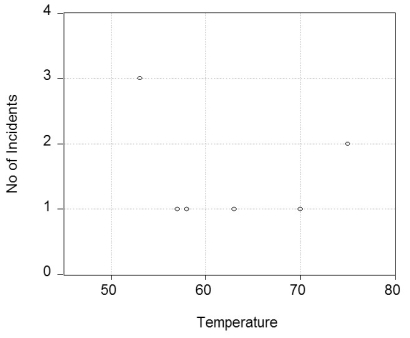(a)Do you see any relationship between the temperature and the number of O-ring failures? If you fitted a linear regression line through these seven observations, do you think the slope would be positive or negative? Significantly different from zero? Do you see any problems other than the sample size in your procedure? (b)You decide to look at all successful launches before Challenger, even those for which there were no incidents. Furthermore you simplify the problem by specifying a binary variable, which takes on the value one if there was some O-ring failure and is zero otherwise. You then fit a linear probability model with the following result, $\widehat{\text { OFail }}$ = 2.858 - 0.037 × Temperature; R² = 0.325, SER = 0.390, (0.496)(0.007) where Ofail is the binary variable which is one for launches where O-rings showed some thermal distress, and Temperature is measured in degrees of Fahrenheit. The numbers in parentheses are heteroskedasticity-robust standard errors. Interpret the equation. Why do you think that heteroskedasticity-robust standard errors were used? What is your prediction for some O-ring thermal distress when the temperature is 31°, the temperature on January 28, 1986? Above which temperature do you predict values of less than zero? Below which temperature do you predict values of greater than one? (c)To fix the problem encountered in (b), you re-estimate the relationship using a logit regression: Pr(OFail = 1 | Temperature)= F (15.297 - 0.236 × Temperature); pseudo- R²=0.297 (7.329)(0.107) What is the meaning of the slope coefficient? Calculate the effect of a decrease in temperature from 80° to 70°, and from 60° to 50°. Why is the change in probability not constant? How does this compare to the linear probability model? (d)You want to see how sensitive the results are to using the logit, rather than the probit estimation method. The probit regression is as follows: Pr(OFail = 1 | Temperature)= Φ(8.900 - 0.137 × Temperature); pseudo- R²=0.296 (3.983)(0.058) Why is the slope coefficient in the probit so different from the logit coefficient? Calculate the effect of a decrease in temperature from 80° to 70°, and from 60° to 50° and compare the resulting changes in probability to your results in (c). What is the meaning of the pseudo- R²? What other measures of fit might you want to consider? (e)Calculate the predicted probability for 80° and 40°, using your probit and logit estimates. Based on the relationship between the probabilities, sketch what the general relationship between the logit and probit regressions is. Does there seem to be much of a difference for values other than these extreme values? (f)You decide to run one more regression, where the dependent variable is the actual number of incidences (NoOFail). You allow for a different functional form by choosing the inverse of the temperature, and estimate the regression by OLS. $\widehat{\text { NoOFail }}$ = -3.8853 + 295.545 × (1/Temperature); R² = 0.386, SER = 0.622 (1.516)(106.541) What is your prediction for O-ring failures for the 31° temperature which was forecasted for the launch on January 28, 1986? Sketch the fitted line of the regression above.

When estimating probit and logit models,