Exam 13: Introduction to Multiple Regression

Instruction 13.20 You worked as an intern at We Always Win Car Insurance Company last summer. You notice that individual car insurance premium depends very much on the age of the individual, the number of traffic tickets received by the individual and the population density of the city in which the individual lives. You performed a regression analysis in Microsoft Excel and obtained the following information: 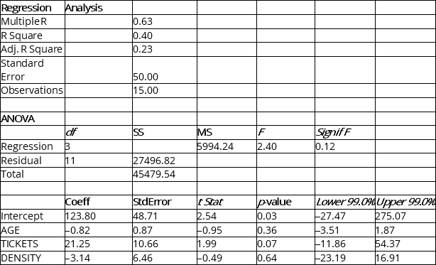-Referring to Instruction 13.20,to test the significance of the multiple regression model,what are the degrees of freedom?

Instruction 13.15 An economist is interested to see how consumption for an economy (in $ billions) is influenced by gross domestic product ($ billions) and aggregate price (consumer price index). The Microsoft Excel output of this regression is partially reproduced below. OUTPUT SUMMARY Regression Statistics MultipleR 0.991 R Square 0.982 Adj. R Square 0.976 Std. Error 0.299 Observations 10 ANOVA df SS MS F Signiff Regression 2 33.4163 16.7082 186.325 0.0001 Residual 7 0.6277 0.0897 Total 9 34.0440 Coeff StdError t Stat p value Intercept -1.6335 0.5674 -0.152 0.8837 GDP 0.7654 0.0574 13.340 0.0001 Price -0.0006 0.0028 -0.219 0.8330 Note: Adj. R Square = Adjusted R Square; Std. Error = Standard Error -Referring to Instruction 13.15,the p-value for GDP is

Instruction 13.21 A weight-loss clinic wants to use regression analysis to build a model for weight-loss of a client (measured in kilograms). Two variables thought to effect weight-loss are client's length of time on the weight loss program and time of session. These variables are described below: Y = Weight-loss (in kilograms) X₁ = Length of time in weight-loss program (in months) X₂ = 1 if morning session, 0 if not X₃ = 1 if afternoon session, 0 if not (Base level = evening session) Data for 12 clients on a weight-loss program at the clinic were collected and used to fit the interaction model: Y = β0 + β₁X₁ + β₂X₂ + β₃X₃ + β₄X₁X₂ + β₅X₁X₃ + ε Partial output from Microsoft Excel follows: -Referring to Instruction 13.21,the overall model for predicting weight-loss (Y)is statistically significant at the 0.05 level.

If you have taken into account all relevant explanatory factors,the residuals from a multiple regression should be random.

Instruction 13.35 The education department's regional executive officer wanted to predict the percentage of students passing a Grade 6 proficiency test. She obtained the data on percentage of students passing the proficiency test (% Passing), daily average of the percentage of students attending class (% Attendance), average teacher salary in dollars (Salaries) and instructional spending per pupil in dollars (Spending) of 47 schools in the state. Following is the multiple regression output with Y = % Passing as the dependent variable, X₁ = % Attendance, X₂ = Salaries and X₃ = Spending: 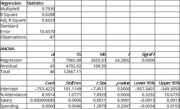-Referring to Instruction 13.35,what is the value of the test statistics when testing whether daily mean of the percentage of students attending class has any effect on percentage of students passing the proficiency test,taking into account the effect of all the other independent variables?

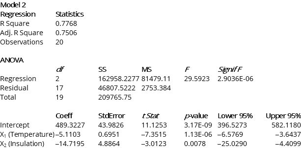
Instruction 13.18 One of the most common questions of prospective house buyers pertains to the average cost of heating in dollars (Y). To provide its customers with information on that matter, a large real estate firm used the following four variables to predict heating costs: the daily minimum outside temperature in degrees of Celsius (X₁), the amount of insulation in cm (X₂), the number of windows in the house (X₃) and the age of the furnace in years (X₄). Given below are the Microsoft Excel outputs of two regression models. 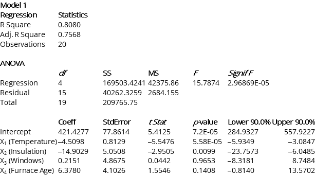-Referring to Instruction 13.18,what can you say about Model 1?

Instruction 13.35 The education department's regional executive officer wanted to predict the percentage of students passing a Grade 6 proficiency test. She obtained the data on percentage of students passing the proficiency test (% Passing), daily average of the percentage of students attending class (% Attendance), average teacher salary in dollars (Salaries) and instructional spending per pupil in dollars (Spending) of 47 schools in the state. Following is the multiple regression output with Y = % Passing as the dependent variable, X₁ = % Attendance, X₂ = Salaries and X₃ = Spending: -Referring to Instruction 13.35,what are the lower and upper limits of the 95% confidence interval estimate for the effect of a one dollar increase in mean teacher salary on the mean percentage of students passing the proficiency test?

Instruction 13.20 You worked as an intern at We Always Win Car Insurance Company last summer. You notice that individual car insurance premium depends very much on the age of the individual, the number of traffic tickets received by the individual and the population density of the city in which the individual lives. You performed a regression analysis in Microsoft Excel and obtained the following information: -Referring to Instruction 13.20,to test the significance of the multiple regression model,the null hypothesis should be rejected while allowing for 1% probability of committing a Type I error.

Instruction 13.23 The Head of the Accounting Department wanted to see if she could predict the average grade of students using the number of course units (credits) and total university entrance exam scores of each. She takes a sample of students and generates the following Microsoft Excel output: OUTPUT SUMMARY Regression Statistics MultipleR 0.916 R Square 0.839 Adj. R Square 0.732 Std. Error 0.24685 Observations 6 ANOVA df SS MS F Signiff Regression 2 0.95219 0.47610 7.813 0.0646 Residual 3 0.18281 0.06094 Total 5 1.13500 Coeff StdError t Stat p value Intercept 4.593897 1.13374542 4.052 0.0271 GDP -0.247270 0.06268485 -3.945 0.0290 Price 0.001443 0.00101241 1.425 0.2494 Note: Adj. R Square = Adjusted R Square; Std. Error = Standard Error -Referring to Instruction 13.23,the Head of Department wants to test H₀: ?₁ = ?₂ = 0.At a level of significance of 0.05,the null hypothesis is rejected.