Exam 13: Introduction to Multiple Regression

Instruction 13.10 The education department's regional executive officer wanted to predict the percentage of students passing a Grade 6 proficiency test. She obtained the data on percentage of students passing the proficiency test (% Passing), daily average of the percentage of students attending class (% Attendance), average teacher salary in dollars (Salaries) and instructional spending per pupil in dollars (Spending) of 47 schools in the state. Following is the multiple regression output with Y = % Passing as the dependent variable, X₁ = % Attendance, X₂ = Salaries and X₃ = Spending: Regression Statistics Multiple R 0.7930 R Square 0.6288 Adj. R Square 0.602 Standard Error 10.4570 Observations 47 ANOVA d SS MS F Signif F Regression 3 7965.08 2655.03 24.2802 0.0000 Residual 43 4702.02 109.35 Total 46 12667.11 Coeff StolFrro tSta p-va/ue Lower 95\% Upper 95\% Intercept -753.4225 101.1149 -7.4511 0.0000 -957.3401 -549.5050 \% Attendance 8.5014 1.0771 7.8929 0.0000 6.3292 10.6735 Salary 0.000000685 0.0006 0.0011 0.9991 -0.0013 0.0013 Spending 0.0060 0.0046 1.2879 0.2047 -0.0034 0.0153 -Referring to Instruction 13.10,which of the following is a correct statement?

Instruction 13.17 A microeconomist wants to determine how corporate sales are influenced by capital and wage spending by companies. She proceeds to randomly select 26 large corporations and record information in millions of dollars. The Microsoft Excel output below shows results of this multiple regression. 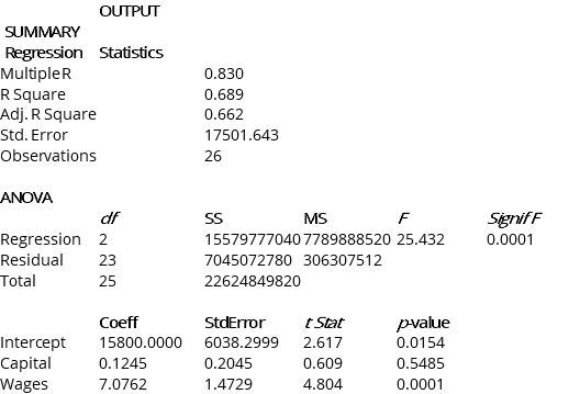Note: Adj. R Square = Adjusted R Square; Std. Error = Standard Error -Referring to Instruction 13.17,which of the following values for α is the smallest for which the regression model as a whole is significant?

Instruction 13.25 Given below are results from the regression analysis where the dependent variable is the number of weeks a worker is unemployed due to a layoff (Unemploy) and the independent variables are the age of the worker (Age), the number of years of education received (Edu), the number of years at the previous job (Job Yr), a dummy variable for marital status (Married: 1 = married, 0 = otherwise), a dummy variable for head of household (Head: 1 = yes, 0 = no) and a dummy variable for management position (Manager: 1 = yes, 0 = no). We shall call this Model 1. Model 1 Regression Statistics Multiple R 0.7035 R Square 0.4949 Adj. R Square 0.4030 Std. Error 18.4861 Observations 40 ANOVA df SS MS F Signiff Regression 6 11048.6415 1841.4402 5.3885 0.00057 Residual 33 11277.2586 341.7351 Total 39 223325.9 Coeff StdError tStat p value Lower 95\% Upper95\% Intercept 32.6595 23.18302 1.4088 0.1683 -14.5067 79.8257 Age 1.2915 0.3599 3.5883 0.0011 0.5592 2.0238 Edu -1.3537 1.1766 -1.1504 0.2582 -3.7476 1.0402 Job Yr 0.6171 0.5940 1.0389 0.3064 -0.5914 1.8257 Married -5.2189 7.6068 -0.6861 0.4974 -20.6950 10.2571 Head -14.2978 7.6479 -1.8695 0.0704 -29.8575 1.2618 Manager -24.8203 11.6932 -2.1226 0.0414 -48.6102 -1.0303 Model 2 is the regression analysis where the dependent variable is Unemploy and the independent variables are Age and Manager. The results of the regression analysis are given below: Mode 2 Regression Statistics Multiple R 0.6391 R Square 0.4085 Adj. R Square 0.3765 Std. Error 18.8929 Observations 40 ANOVA df SS MS F Signiff Regression 2 9119.0897 4559.5448 12.7740 0.0000 Residual 37 13206.8103 356.9408 Total 39 22325.9 Coeff StdError t Stat p value Intercept -0.2143 11.5796 -0.0185 0.9853 Age 1.4448 0.3160 4.5717 0.0000 Manager -22.5761 11.3488 -1.9893 0.0541 -Referring to Instruction 13.25 Model 1,the null hypothesis H₀: ?₁ = ?₂ = ?₃ = ?₄ = ?₅ = ?₆ = 0 implies that the number of weeks a worker is unemployed due to a layoff is not affected by some of the explanatory variables.

If a categorical independent variable contains four categories,then ___________ dummy variable(s)will be needed to uniquely represent these categories.

AU: Question 37 is the same as Question 36. Please check. Instruction 13.12 AU: Please advise if Instruction 13.12 can be renumbered to Instruction 13.11 and further questions renumbered. Or advise whether there shall be new Instruction 13.11 included. The Head of the Accounting Department wanted to see if she could predict the average grade of students using the number of course units (credits) and total university entrance exam scores of each. She takes a sample of students and generates the following Microsoft Excel output: OUTPUT SUMMARY Regression Statistics MultipleR 0.916 R Square 0.839 Adj. R Square 0.732 Std. Error 0.24685 Observations 6 ANOVA df SS MS F Signiff Regression 2 0.95219 0.47610 7.813 0.0646 Residual 3 0.18281 0.06094 Total 5 1.13500 Coeff StdError t Stat p value Intercept 4.593897 1.13374542 4.052 0.0271 GDP -0.247270 0.06268485 -3.945 0.0290 Price 0.001443 0.00101241 1.425 0.2494 Note: Adj. R Square = Adjusted R Square; Std. Error = Standard Error -Referring to Instruction 13.12,the value of the coefficient of multiple determination,r²_Y.12,is ___________.

AU: Question 37 is the same as Question 36. Please check. Instruction 13.12 AU: Please advise if Instruction 13.12 can be renumbered to Instruction 13.11 and further questions renumbered. Or advise whether there shall be new Instruction 13.11 included. The Head of the Accounting Department wanted to see if she could predict the average grade of students using the number of course units (credits) and total university entrance exam scores of each. She takes a sample of students and generates the following Microsoft Excel output: OUTPUT SUMMARY Regression Statistics MultipleR 0.916 R Square 0.839 Adj. R Square 0.732 Std. Error 0.24685 Observations 6 ANOVA df SS MS F Signiff Regression 2 0.95219 0.47610 7.813 0.0646 Residual 3 0.18281 0.06094 Total 5 1.13500 Coeff StdError t Stat p value Intercept 4.593897 1.13374542 4.052 0.0271 GDP -0.247270 0.06268485 -3.945 0.0290 Price 0.001443 0.00101241 1.425 0.2494 Note: Adj. R Square = Adjusted R Square; Std. Error = Standard Error -Referring to Instruction 13.12,the Head of Department wants to test H₀: $\beta$ ₁ = $\beta$ ₂ = 0.The appropriate alternative hypothesis is ___________.

Instruction 13.31 A microeconomist wants to determine how corporate sales are influenced by capital and wage spending by companies. She proceeds to randomly select 26 large corporations and record information in millions of dollars. The Microsoft Excel output below shows results of this multiple regression. Note: Adj. R Square = Adjusted R Square; Std. Error = Standard Error -Referring to Instruction 13.31,suppose the microeconomist wants to test whether the coefficient on Capital is significantly different from 0.What is the value of the relevant t-statistic?

Instruction 13.22 The education department's regional executive officer wanted to predict the percentage of students passing a Grade 6 proficiency test. She obtained the data on percentage of students passing the proficiency test (% Passing), daily average of the percentage of students attending class (% Attendance), average teacher salary in dollars (Salaries) and instructional spending per pupil in dollars (Spending) of 47 schools in the state. Following is the multiple regression output with Y = % Passing as the dependent variable, X₁ = % Attendance, X₂ = Salaries and X₃ = Spending: 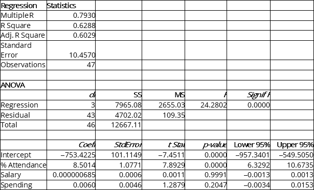-Referring to Instruction 13.22,you can conclude that instructional spending per pupil has no impact on mean percentage of students passing the proficiency test at a 10% level of significance based solely on the 95% confidence interval estimate for β₃.

Instruction 13.22 The education department's regional executive officer wanted to predict the percentage of students passing a Grade 6 proficiency test. She obtained the data on percentage of students passing the proficiency test (% Passing), daily average of the percentage of students attending class (% Attendance), average teacher salary in dollars (Salaries) and instructional spending per pupil in dollars (Spending) of 47 schools in the state. Following is the multiple regression output with Y = % Passing as the dependent variable, X₁ = % Attendance, X₂ = Salaries and X₃ = Spending: -Referring to Instruction 13.22,the alternative hypothesis H₁: At least one of β_j ≠ 0 for j = 1,2,3 implies that percentage of students passing the proficiency test is related to at least one of the explanatory variables.

Instruction 13.34 An automotive engineer would like to be able to predict automobile fuel economy. She believes that the two most important characteristics that affect economy are engine power and the number of cylinders (4 or 6) of a car. She believes that the appropriate model is Y=40-0.05+20-0.1 where = engine power =1 if 4 cylinders, 0 if 6 cylinders Y = economy expressed as kilometres. -Referring to Instruction 13.34,the predicted number of kilometres for a 200 engine power,4-cylinder car is ___________.

Instruction 13.37 Given below are results from the regression analysis where the dependent variable is the number of weeks a worker is unemployed due to a layoff (Unemploy) and the independent variables are the age of the worker (Age), the number of years of education received (Edu), the number of years at the previous job (Job Yr), a dummy variable for marital status (Married: 1 = married, 0 = otherwise), a dummy variable for head of household (Head: 1 = yes, 0 = no) and a dummy variable for management position (Manager: 1 = yes, 0 = no). We shall call this Model 1. Model 1 Regression Statistics Multiple R 0.7035 R Square 0.4949 Adj. R Square 0.4030 Std. Error 18.4861 Observations 40 ANOVA df SS MS F Signif F Regression 6 11048.6415 1841.4402 5.3885 0.00057 Residual 33 11277.2586 341.7351 Total 39 223325.9 Coeff StdError tStat p value Lower 95\% Upper95\% Intercept 32.6595 23.18302 1.4088 0.1683 -14.5067 79.8257 Age 1.2915 0.3599 3.5883 0.0011 0.5592 2.0238 Edu -1.3537 1.1766 -1.1504 0.2582 -3.7476 1.0402 Job Yr 0.6171 0.5940 1.0389 0.3064 -0.5914 1.8257 Married -5.2189 7.6068 -0.6861 0.4974 -20.6950 10.2571 Head -14.2978 7.6479 -1.8695 0.0704 -29.8575 1.2618 Manager -24.8203 11.6932 -2.1226 0.0414 -48.6102 -1.0303 Model 2 is the regression analysis where the dependent variable is Unemploy and the independent variables are Age and Manager. The results of the regression analysis are given below: Mode 2 Regression Statistics Multiple R 0.6391 R Square 0.4085 Adj. R Square 0.3765 Std. Error 18.8929 Observations 40 ANOVA df SS MS F Signif F Regression 2 9119.0897 4559.5448 12.7740 0.0000 Residual 37 13206.8103 356.9408 Total 39 22325.9 Coeff StdError t Stat p value Intercept -0.2143 11.5796 -0.0185 0.9853 Age 1.4448 0.3160 4.5717 0.0000 Manager -22.5761 11.3488 -1.9893 0.0541 -Referring to Instruction 13.37 Model 1,what are the lower and upper limits of the 95% confidence interval estimate for the difference in the mean number of weeks a worker is unemployed due to a layoff between a worker who is married and one who is not after taking into consideration the effect of all the other independent variables?

Instruction 13.32 One of the most common questions of prospective house buyers pertains to the average cost of heating in dollars (Y). To provide its customers with information on that matter, a large real estate firm used the following four variables to predict heating costs: the daily minimum outside temperature in degrees of Celsius (X₁), the amount of insulation in cm (X₂), the number of windows in the house (X₃) and the age of the furnace in years (X₄). Given below are the Microsoft Excel outputs of two regression models. 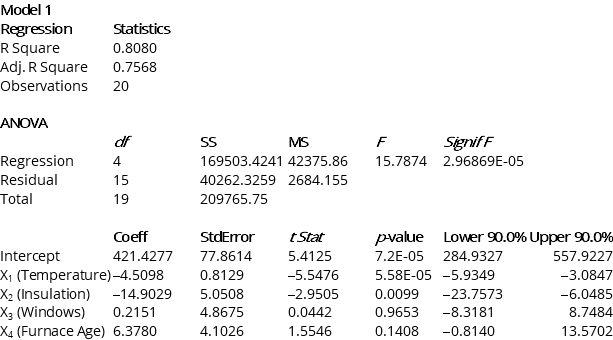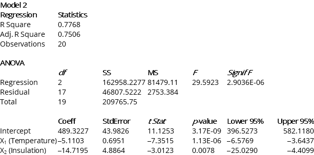-Referring to Instruction 13.32,what is the 90% confidence interval for the expected change in heating costs as a result of a 1 degree Celsius change in the daily minimum outside temperature using Model 1?

Instruction 13.2 A lecturer in industrial relations believes that an individual's wage rate at a factory (Y) depends on his performance rating (X₁) and the number of economics courses the employee successfully completed at university (X₂). The lecturer randomly selects six workers and collects the following information: Employee Y(\ ) X1 X2 1 10 3 0 2 12 1 5 3 15 8 1 4 17 5 8 5 20 7 12 6 25 10 9 -Referring to Instruction 13.2,for these data,what is the estimated coefficient for performance rating,b₁?

Instruction 13.25 Given below are results from the regression analysis where the dependent variable is the number of weeks a worker is unemployed due to a layoff (Unemploy) and the independent variables are the age of the worker (Age), the number of years of education received (Edu), the number of years at the previous job (Job Yr), a dummy variable for marital status (Married: 1 = married, 0 = otherwise), a dummy variable for head of household (Head: 1 = yes, 0 = no) and a dummy variable for management position (Manager: 1 = yes, 0 = no). We shall call this Model 1. Model 1 Regression Statistics Multiple R 0.7035 R Square 0.4949 Adj. R Square 0.4030 Std. Error 18.4861 Observations 40 ANOVA df SS MS F Signiff Regression 6 11048.6415 1841.4402 5.3885 0.00057 Residual 33 11277.2586 341.7351 Total 39 223325.9 Coeff StdError tStat p value Lower 95\% Upper95\% Intercept 32.6595 23.18302 1.4088 0.1683 -14.5067 79.8257 Age 1.2915 0.3599 3.5883 0.0011 0.5592 2.0238 Edu -1.3537 1.1766 -1.1504 0.2582 -3.7476 1.0402 Job Yr 0.6171 0.5940 1.0389 0.3064 -0.5914 1.8257 Married -5.2189 7.6068 -0.6861 0.4974 -20.6950 10.2571 Head -14.2978 7.6479 -1.8695 0.0704 -29.8575 1.2618 Manager -24.8203 11.6932 -2.1226 0.0414 -48.6102 -1.0303 Model 2 is the regression analysis where the dependent variable is Unemploy and the independent variables are Age and Manager. The results of the regression analysis are given below: Mode 2 Regression Statistics Multiple R 0.6391 R Square 0.4085 Adj. R Square 0.3765 Std. Error 18.8929 Observations 40 ANOVA df SS MS F Signiff Regression 2 9119.0897 4559.5448 12.7740 0.0000 Residual 37 13206.8103 356.9408 Total 39 22325.9 Coeff StdError t Stat p value Intercept -0.2143 11.5796 -0.0185 0.9853 Age 1.4448 0.3160 4.5717 0.0000 Manager -22.5761 11.3488 -1.9893 0.0541 -Referring to Instruction 13.25 Model 1,which of the following is the correct null hypothesis to determine whether there is a significant relationship between the number of weeks a worker is unemployed due to a layoff and the entire set of explanatory variables?

Instruction 13.23 The Head of the Accounting Department wanted to see if she could predict the average grade of students using the number of course units (credits) and total university entrance exam scores of each. She takes a sample of students and generates the following Microsoft Excel output: OUTPUT SUMMARY Regression Statistics MultipleR 0.916 R Square 0.839 Adj. R Square 0.732 Std. Error 0.24685 Observations 6 ANOVA df SS MS F Signiff Regression 2 0.95219 0.47610 7.813 0.0646 Residual 3 0.18281 0.06094 Total 5 1.13500 Coeff StdError t Stat p value Intercept 4.593897 1.13374542 4.052 0.0271 GDP -0.247270 0.06268485 -3.945 0.0290 Price 0.001443 0.00101241 1.425 0.2494 Note: Adj. R Square = Adjusted R Square; Std. Error = Standard Error -Referring to Instruction 13.23,the Head of Department wants to use a t test to test for the significance of the coefficient of X₁.The value of the test statistic is _____.

Instruction 13.25 Given below are results from the regression analysis where the dependent variable is the number of weeks a worker is unemployed due to a layoff (Unemploy) and the independent variables are the age of the worker (Age), the number of years of education received (Edu), the number of years at the previous job (Job Yr), a dummy variable for marital status (Married: 1 = married, 0 = otherwise), a dummy variable for head of household (Head: 1 = yes, 0 = no) and a dummy variable for management position (Manager: 1 = yes, 0 = no). We shall call this Model 1. Model 1 Regression Statistics Multiple R 0.7035 R Square 0.4949 Adj. R Square 0.4030 Std. Error 18.4861 Observations 40 ANOVA df SS MS F Signiff Regression 6 11048.6415 1841.4402 5.3885 0.00057 Residual 33 11277.2586 341.7351 Total 39 223325.9 Coeff StdError tStat p value Lower 95\% Upper95\% Intercept 32.6595 23.18302 1.4088 0.1683 -14.5067 79.8257 Age 1.2915 0.3599 3.5883 0.0011 0.5592 2.0238 Edu -1.3537 1.1766 -1.1504 0.2582 -3.7476 1.0402 Job Yr 0.6171 0.5940 1.0389 0.3064 -0.5914 1.8257 Married -5.2189 7.6068 -0.6861 0.4974 -20.6950 10.2571 Head -14.2978 7.6479 -1.8695 0.0704 -29.8575 1.2618 Manager -24.8203 11.6932 -2.1226 0.0414 -48.6102 -1.0303 Model 2 is the regression analysis where the dependent variable is Unemploy and the independent variables are Age and Manager. The results of the regression analysis are given below: Mode 2 Regression Statistics Multiple R 0.6391 R Square 0.4085 Adj. R Square 0.3765 Std. Error 18.8929 Observations 40 ANOVA df SS MS F Signiff Regression 2 9119.0897 4559.5448 12.7740 0.0000 Residual 37 13206.8103 356.9408 Total 39 22325.9 Coeff StdError t Stat p value Intercept -0.2143 11.5796 -0.0185 0.9853 Age 1.4448 0.3160 4.5717 0.0000 Manager -22.5761 11.3488 -1.9893 0.0541 -Referring to Instruction 13.25 Model 1,the null hypothesis H₀: ?₁ = ?₂ = ?₃ = ?₄ = ?₅ = ?₆ = 0 implies that the number of weeks a worker is unemployed due to a layoff is not related to any of the explanatory variables.

Instruction 13.37 Given below are results from the regression analysis where the dependent variable is the number of weeks a worker is unemployed due to a layoff (Unemploy) and the independent variables are the age of the worker (Age), the number of years of education received (Edu), the number of years at the previous job (Job Yr), a dummy variable for marital status (Married: 1 = married, 0 = otherwise), a dummy variable for head of household (Head: 1 = yes, 0 = no) and a dummy variable for management position (Manager: 1 = yes, 0 = no). We shall call this Model 1. Model 1 Regression Statistics Multiple R 0.7035 R Square 0.4949 Adj. R Square 0.4030 Std. Error 18.4861 Observations 40 ANOVA df SS MS F Signif F Regression 6 11048.6415 1841.4402 5.3885 0.00057 Residual 33 11277.2586 341.7351 Total 39 223325.9 Coeff StdError tStat p value Lower 95\% Upper95\% Intercept 32.6595 23.18302 1.4088 0.1683 -14.5067 79.8257 Age 1.2915 0.3599 3.5883 0.0011 0.5592 2.0238 Edu -1.3537 1.1766 -1.1504 0.2582 -3.7476 1.0402 Job Yr 0.6171 0.5940 1.0389 0.3064 -0.5914 1.8257 Married -5.2189 7.6068 -0.6861 0.4974 -20.6950 10.2571 Head -14.2978 7.6479 -1.8695 0.0704 -29.8575 1.2618 Manager -24.8203 11.6932 -2.1226 0.0414 -48.6102 -1.0303 Model 2 is the regression analysis where the dependent variable is Unemploy and the independent variables are Age and Manager. The results of the regression analysis are given below: Mode 2 Regression Statistics Multiple R 0.6391 R Square 0.4085 Adj. R Square 0.3765 Std. Error 18.8929 Observations 40 ANOVA df SS MS F Signif F Regression 2 9119.0897 4559.5448 12.7740 0.0000 Residual 37 13206.8103 356.9408 Total 39 22325.9 Coeff StdError t Stat p value Intercept -0.2143 11.5796 -0.0185 0.9853 Age 1.4448 0.3160 4.5717 0.0000 Manager -22.5761 11.3488 -1.9893 0.0541 -Referring to Instruction 13.37 Model 1,what is the p-value of the test statistic to determine whether there is a significant relationship between the number of weeks a worker is unemployed due to a layoff and the entire set of explanatory variables?

Instruction 13.20 You worked as an intern at We Always Win Car Insurance Company last summer. You notice that individual car insurance premium depends very much on the age of the individual, the number of traffic tickets received by the individual and the population density of the city in which the individual lives. You performed a regression analysis in Microsoft Excel and obtained the following information: 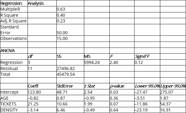-Referring to Instruction 13.20,the 99% confidence interval for the change in average insurance premiums of a person who has become one year older (i.e.,the slope coefficient for AGE)is _____.

Instruction 13.30 A real estate builder wishes to determine how house size (House) is influenced by family income (Income), family size (Size) and education of the head of household (School). House size is measured in hundreds of square metres, income is measured in thousands of dollars and education is in years. The builder randomly selected 50 families and ran the multiple regression. Microsoft Excel output is provided below: OUTPUT SUMMARY Regression Statistics Multiple R 0.865 R Square 0.748 Adj. R Square 0.726 Std. Error 5.195 Observations 50 ANOVA df SS MS F Signiff Regression 3605.7736 901.4434 0.0001 Residual 1214.2264 26.9828 Total 49 4820.0000 Coeff StdError t Stat p value Intercept -1.6335 5.8078 -0.281 0.7798 Income 0.4485 0.1137 3.9545 0.0003 Size 4.2615 0.8062 5.286 0.0001 School -0.6517 0.4319 -1.509 0.1383 Note: Adj. R Square = Adjusted R Square; Std. Error = Standard Error -Referring to Instruction 13.30,the observed value of the F statistic is missing from the printout.What are the degrees of freedom for this F statistic?

Instruction 13.1 A manager of a product sales group believes the number of sales made by an employee (Y) depends on how many years that employee has been with the company (X₁) and how he/she scored on a business aptitude test (X₂). A random sample of 8 employees provides the following: Employee Y X1 X2 1 100 10 7 2 90 3 10 3 80 8 9 4 70 5 4 5 60 5 8 6 50 7 5 7 40 1 4 8 30 1 1 -Referring to Instruction 13.1,if an employee who had been with the company for five years scored a 9 on the aptitude test,what would his estimated expected sales be?