Exam 4: Sensitivity Analysis and the Simplex Method
Exam 1: Introduction to Modeling and Decision Analysis74 Questions
Exam 2: Introduction to Optimization and Linear Programming73 Questions
Exam 3: Modeling and Solving Lp Problems in a Spreadsheet75 Questions
Exam 4: Sensitivity Analysis and the Simplex Method77 Questions
Exam 5: Network Modeling84 Questions
Exam 6: Integer Linear Programming88 Questions
Exam 7: Goal Programming and Multiple Objective Optimization65 Questions
Exam 8: Nonlinear Programming and Evolutionary Optimization69 Questions
Exam 9: Regression Analysis82 Questions
Exam 10: Data Mining102 Questions
Exam 11: Time Series Forecasting81 Questions
Exam 12: Introduction to Simulation Using Analytic Solver Platform70 Questions
Exam 13: Queuing Theory87 Questions
Exam 14: Decision Analysis116 Questions
Exam 15: Project Management Online65 Questions
Select questions type
Exhibit 4.1
The following questions are based on the problem below and accompanying Analytic Solver Platform sensitivity report.
Carlton construction is supplying building materials for a new mall construction project in Kansas.Their contract calls for a total of 250,000 tons of material to be delivered over a three-week period.Carlton's supply depot has access to three modes of transportation: a trucking fleet,railway delivery,and air cargo transport.Their contract calls for 120,000 tons delivered by the end of week one,80% of the total delivered by the end of week two,and the
entire amount delivered by the end of week three.Contracts in place with the transportation companies call for at least 45% of the total delivered be delivered by trucking,at least 40% of the total delivered be delivered by railway,and up to 15% of the total delivered be delivered by air cargo.Unfortunately,competing demands limit the availability of each mode of transportation each of the three weeks to the following levels all in thousands of tons):
Week TruckingLimits Railway Limits Air Cargo Limits 1 45 60 15 2 50 55 10 3 55 45 5 Costs \ per 1000 tons) \ 200 \ 140 \ 400
The following is the LP model for this logistics problem.
Let Xij = amount shipped by mode i in week j
where i = 1Truck),2Rail),3Air)and j = 1,2,3
Let WLij = weekly limit of mode i in week j as provided in above table)
200X11 + X12 + X13)+ 140X21 + X22 + X23)+ 500X31 +
MIN:
X + X )
Subject to:
32 33
Xij ? WL ij for all i and j Weekly limits by mode
X11 + X12 + X13 + X21 + X22 + X23 + X31 + X32 + X33 ? 250
Total at end of three weeks
X11 + X21 + X31 + X12 + X22 + X32 ? 200 Total at end of two weeks X11 + X21 + X31 ? 120 Total at end of first week
X11 + X12 + X13 ? 0.45*250 Truck mix requirement
X21 + X22 + X23 ? 0.40*250 Rail mix requirement
X31 + X32 + X33 ? 0.15*250 Air mix limit Xij ? 0 for all i and j
Final Reduced Objective Allowable Allowable Value Cost Coefficient Increase Decrease Cell Name \ \ 6 Week 1 by Truck 45 0 200 360 1+30 \ \ 6 Week 1 by Rail 60 0 140 360 1+30 \ \ 6 Week 1 by Air 15 0 500 1+30 360 \ \ 7 Week 2 by Truck 50 0 200 0 1+30 \ \ 7 Week 2 by Rail 55 0 140 0 1+30 \ \ 7 Week 2 by Air 0 360 500 1+30 360 \ \ 8 Week 3 by Truck 13 0 200 1+30 0 \ \ 8 Week 3 by Rail 12 0 140 60 0 \ F\ 8 Week 3 by Air 0 360 500 1+30 360
 -Refer to Exhibit 4.1.The Week 1 by Truck and Week 1 by Rail constraints each have a shadow price of ?360.
What do these values imply?
-Refer to Exhibit 4.1.The Week 1 by Truck and Week 1 by Rail constraints each have a shadow price of ?360.
What do these values imply?
(Essay)
4.7/5  (34)
(34)
To convert ≤ constraints into = constraints the Simplex method adds what type of variable to the constraint?
(Multiple Choice)
4.9/5 (38)
The slope of the level curve for the objective function value can be changed by
(Multiple Choice)
4.8/5 (30)
A farmer is planning his spring planting.He has 20 acres on which he can plant a combination of Corn,Pumpkins and Beans.He wants to maximize his profit but there is a limited demand for each crop.Each crop also requires fertilizer and irrigation water which are in short supply.The following table summarizes the data for the problem.
Suppose the farmer can purchase more fertilizer for $2.50 per pound,should he purchase it and how much can he buy and still be sure of the value of the additional fertilizer? Base your response on the following Analytic Solver Platform sensitivity output.
Cell Name Final Value Reduced Cost Objective Coefficient Allowable Increase Allowable Decrease \ \ 4 Acres of Corn 9.52 0 2100 1+30 350 \ \ 4 Acres of Pumpkin 0 -500.01 899.99 500.01 1+30 \ \ 4 Acres of Beans 10.79 0 1050 210 375.00
Cell Name Final Value Shadow Price Constraint R.H. Side Allowable Increase Allowable Decrease \ E\ 8 Com demand Used 200000 0.017 200000 136000 152000 \ E\ 9 Pumplin demand Used 0 0 180000 1E+30 180000 \ E\ 10 Bean demand Used 37777.78 0 80000 1+30 42222.22 \ E\ 11 Water Used 29.84 0 50 1E+30 20.15 \F \1 2 Fertilizer IJsed 8000 35 8000 3619.04 3238.09
(Essay)
4.8/5 (23)
For a minimization problem,if a decision variable's final value is 0,and its reduced cost is negative,which of the following is true?
(Multiple Choice)
4.7/5 (43)
If the shadow price for a resource is 0 and 150 units of the resource are added what happens to the optimal solution?
(Multiple Choice)
4.7/5 (28)
Consider the formulation below.The standard form of the second constraint is:
MAX: 8 X1 + 4 X2
Subject to: 5 X1 + 5 X2 ≤ 20
6 X1 + 2 X2 ≥ 18
X1,X2 ≥ 0
(Multiple Choice)
4.8/5 (29)
The difference between the right-hand side RHS)values of the constraints and the final optimal)value assumed by the left-hand side LHS)formula for each constraint is called the slack and is found in the
(Multiple Choice)
4.9/5 (36)
What is the smallest value of the objective function coefficient X1 can assume without changing the optimal solution?
MAX: 7 X1 + 4 X2
Subject to: 2 X1 + X2 ≤ 16
X1 + X2 ≤ 10
2 X1 + 5 X2 ≤ 40 X1,X2 ≥ 0

(Essay)
4.8/5 (38)
The absolute value of the shadow price indicates the amount by which the objective function will be
(Multiple Choice)
4.8/5 (35)
Use slack variables to rewrite this problem so that all its constraints are equality constraints.
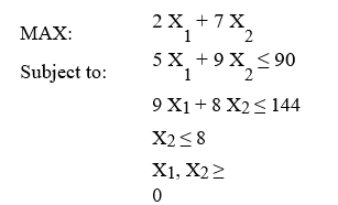
(Essay)
4.8/5 (40)
Why might a decision maker prefer a solution in the interior of the feasible region of a linear programming problem?
(Multiple Choice)
4.8/5 (40)
When performing sensitivity analysis,which of the following assumptions must apply?
(Multiple Choice)
4.9/5 (37)
Consider the following linear programming model and Analytic Solver Platform sensitivity output.What is the optimal objective function value if the RHS of the first constraint increases to 18?
MAX: 7 X1 + 4 X2
Subject to: 2 X1 + X2 ≤ 16
X1 + X2 ≤ 10
2 X1 + 5 X2 ≤ 40 X1,X2 ≥ 0

(Essay)
4.9/5 (29)
What are the objective function coefficients for X1 and X2 based on the following Analytic Solver Platform sensitivity output?
Cell Target Name Value \E \5 Unit profit: OBJ. FN. VALUE 58
Cell Adjustable Name Value Lower Limit Target Result Upper Limit Target Result \ \ 4 Number to make: 1 6 0 16 6 58 \ \ 4 Number to make: 2 4 0 42 4 58
(Essay)
4.9/5 (43)
A binding greater than or equal to ≥)constraint in a minimization problem means that
(Multiple Choice)
4.8/5 (25)
A solution to the system of equations using a set of basic variables is called
(Multiple Choice)
4.8/5 (34)
Solve this problem graphically.What is the optimal solution and what constraints are binding at the optimal solution?
MIN: 7 X1 + 3 X2
Subject to: 4 X1 + 4 X2 ≥ 40
2 X1 + 3 X2 ≥ 24 X1,X2 ≥ 0
(Essay)
4.8/5 (48)
Filters
- Essay(0)
- Multiple Choice(0)
- Short Answer(0)
- True False(0)
- Matching(0)