Exam 13: Inference for Regression

Forced expiratory volume (FEV) is the volume of exhaled air, and it is related to lung size as well as to lung function. FEV is typically lower in persons with impaired lung function due to disease. The residual plots below are from two regressions: the first plot is from regressing height on FEV and the second is from regressing height on log(FEV). 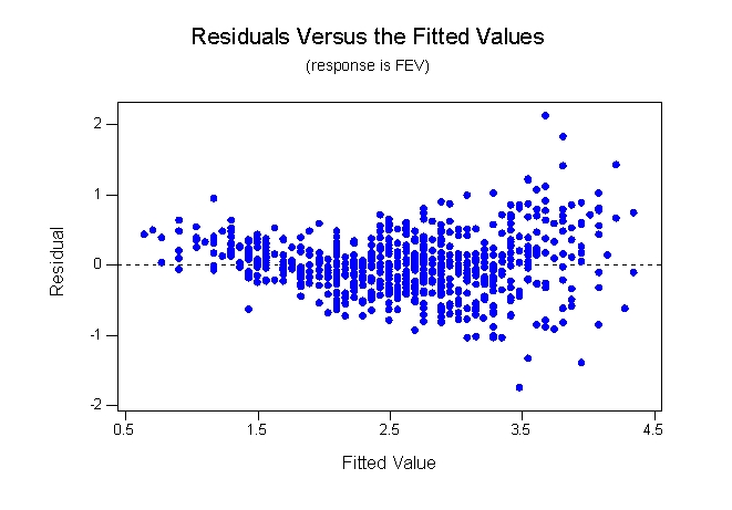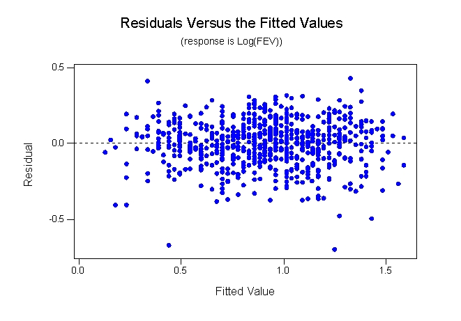Based on these plots, which statement is correct?

A study of obesity risk in children in a head start program used a food score calculated from a 45-question food survey to predict body mass index (BMI) percentile in these children 18 months after the initial survey. The study enrolled 20 children. The researchers used a linear regression model for the prediction of BMI percentile. The food scores ranged from 45 to 245. The residual plot below was obtained by the researchers. 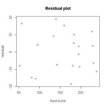The plot does not show any obvious model violations because:

A random sample of 19 companies from the Forbes 500 list was selected, and the relationship between sales (in hundreds of thousands of dollars) and profits (in hundreds of thousands of dollars) was investigated by regression. The following simple linear regression model was used: profits =  +  (sales), where the deviations were assumed to be independent and Normally distributed, with mean 0 and standard deviation . This model was fit to the data using the method of least squares. The following results were obtained from statistical software. r² = 0.662 S = 466.2 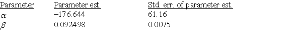Is there evidence of a straight-line relationship between sales and profits?

You can visit the official website of any large restaurant chain to examine the nutritional data for menu items. For fast-food restaurants, many menu items are high in fat, so most of their calorie content comes from fat (rather than from carbohydrates or protein). Here we investigate the relationship between the amount of fat in a menu item (in grams) and the number of calories. To predict the number of calories in a menu item given its fat content, we use the simple linear regression model calories =  +  (fat), where the deviations are assumed to be independent and Normally distributed, with mean 0 and standard deviation . At one major fast-food restaurant chain, there were 26 items listed under the heading of "Sandwiches" (which includes hamburgers, chicken sandwiches, and other sandwich selections) on the menu. We fit the model to the data using the method of least squares. We treat these 26 menu items (which came from one restaurant) as a sample from the population of all sandwich items at all fast-food restaurants. Suppose the researchers test the hypotheses H₀:  = 0, H_a:  > 0. The value of the t statistic for this test is greater than 5. The P-value corresponding to the test of the hypotheses is:

Frequent food questionnaires (FFQs) are often given to large groups of people to obtain information on their dietary habits. Study participants are asked about the frequency with which they consume certain goods. Another method to obtain information on foods consumed is a food diary. People are asked to record every type of food and amount consumed for a few days. Food diaries are more difficult to obtain and response rates are lower than for FFQs. A study was conducted to see how well FFQs predict food consumed based on food diaries. In this study, the explanatory variable is:

A study of obesity risk in children in a head start program used a food score calculated from a 45-question food survey to predict body mass index (BMI) percentile in these children 18 months after the initial survey. The study enrolled 20 children. The researchers used a linear regression model for the prediction of BMI percentile. The food scores ranged from 45 to 245. The linear regression had slope = 0.29 and intercept = 18.3. The average BMI percentile for a child with food score 150 equals 61.8, and an individual child with food score 150 will be predicted to have a BMI percentile of:

A study of obesity risk in children in a head start program used a food score calculated from a 45-question food survey to predict body mass index (BMI) percentile in these children 18 months after the initial survey. The study enrolled 20 children. The researchers used a linear regression model for the prediction of BMI percentile. The food scores ranged from 45 to 245. The least-squares estimate for the slope was 0.29 with standard error SE = 0.046. The t statistic for the hypothesis H₀:  = 0 is given by:

A study of obesity risk in children in a head start program used a food score calculated from a 45-question food survey to predict body mass index (BMI) percentile in these children 18 months after the initial survey. The study enrolled 20 children. The researchers used a linear regression model for the prediction of BMI percentile. The food scores ranged from 45 to 245. 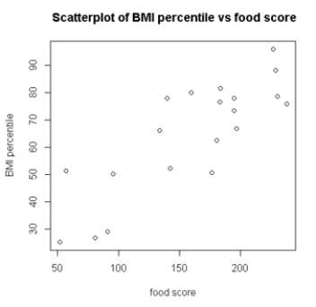Which feature, supported by the scatterplot, is important to determine if a linear regression model can be used?

A study of obesity risk in children in a head start program used a food score calculated from a 45-question food survey to predict body mass index (BMI) percentile in these children 18 months after the initial survey. The study enrolled 20 children. The researchers used a linear regression model for the prediction of BMI percentile. The food scores ranged from 45 to 245. Two computer programs the researchers used to obtain their regression model and related calculations also provided two intervals for a child with food score 150. Interval I₁ = (56.13, 67.35) and interval I₂ = (36.35, 87.13). These intervals, respectively, are called:

A random sample of 19 companies from the Forbes 500 list was selected, and the relationship between sales (in hundreds of thousands of dollars) and profits (in hundreds of thousands of dollars) was investigated by regression. The following simple linear regression model was used: profits =  +  (sales), where the deviations were assumed to be independent and Normally distributed, with mean 0 and standard deviation . This model was fit to the data using the method of least squares. The following results were obtained from statistical software. r² = 0.662 S = 466.2 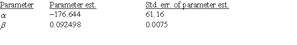Suppose the researchers test the hypotheses H₀: ₁ = 0, H_a: ₁ > 0. The P-value of the test is:

A random sample of 19 companies from the Forbes 500 list was selected, and the relationship between sales (in hundreds of thousands of dollars) and profits (in hundreds of thousands of dollars) was investigated by regression. The following simple linear regression model was used: profits =  +  (sales), where the deviations were assumed to be independent and Normally distributed, with mean 0 and standard deviation . This model was fit to the data using the method of least squares. The following results were obtained from statistical software. r² = 0.662 S = 466.2 The approximate slope of the least-squares regression line is:

The scatterplot below suggests a linear relationship between the age (in years) of an antique clock and its sale price (in euros) at auction. The data are age and sale price for 11 antique clocks sold at a recent auction. We fit the least-squares regression line to the model price =  +  (age), where the deviations are assumed to be independent and Normally distributed, with mean 0 and standard deviation . A summary of the output is given. r² = 0.848 S = 33.1559 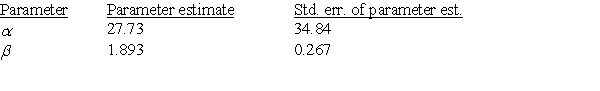The correlation between the age of the antique clock and the auction price of the antique clock is:

The scatterplot below suggests a linear relationship between the age (in years) of an antique clock and its sale price (in euros) at auction. The data are age and sale price for 11 antique clocks sold at a recent auction. 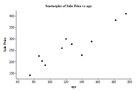We fit the least-squares regression line to the model price =  +  (age), where the deviations are assumed to be independent and Normally distributed, with mean 0 and standard deviation . A summary of the output is given. r² = 0.848 S = 33.1559 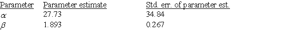An approximate 95% confidence interval for the slope  in the simple linear regression model is:

The scatterplot below suggests a linear relationship between the age (in years) of an antique clock and its sale price (in euros) at auction. The data are age and sale price for 11 antique clocks sold at a recent auction. We fit the least-squares regression line to the model price =  +  (age), where the deviations are assumed to be independent and Normally distributed, with mean 0 and standard deviation . A summary of the output is given. r² = 0.848 S = 33.1559 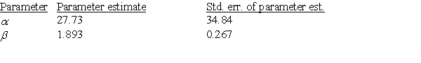Suppose the researchers test the hypotheses H₀:  = 0, H_a:   0. The value of the t statistic for this test is:

The following is a scatterplot of a company's profits versus their sales (in dollars). Each point on the plot represents profits and sales during one of the months in the sample. 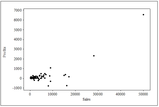What should you do about the two points that represent profits for sales of $20K or more?

Forced expiratory volume (FEV) is the volume of exhaled air and is related to lung size as well as lung function. It is typically lower in persons with impaired lung function due to disease. A regression of height (in inches) on FEV (in liters) showed a nonlinear pattern. Therefore, height was regressed on log(FEV) (natural log) and the residual plot showed a much improved fit. The intercept a and slope b from the regression of height on log(FEV) are a = -2.2 and b = 0.06. A 5-foot-tall person is predicted to have a lung volume of:

The following is a scatterplot of a company's profits versus their sales (in dollars). Each point on the plot represents profits and sales during one of the months in the sample. Which of the following statements is supported by the plot?

A study of obesity risk in children in a head start program used a food score calculated from a 45-question food survey to predict body mass index (BMI) percentile in these children 18 months after the initial survey. The study enrolled 20 children. The researchers used a linear regression model for the prediction of BMI percentile. The food scores ranged from 45 to 245. The regression line that is calculated by standard regression programs or by hand is called the least-squares line because it:

You can visit the official website of any large restaurant chain to examine the nutritional data for menu items. For fast-food restaurants, many menu items are high in fat, so most of their calorie content comes from fat (rather than from carbohydrates or protein). Here we investigate the relationship between the amount of fat in a menu item (in grams) and the number of calories. To predict the number of calories in a menu item given its fat content, we use the simple linear regression model calories =  +  (fat), where the deviations are assumed to be independent and Normally distributed, with mean 0 and standard deviation . At one major fast-food restaurant chain, there were 26 items listed under the heading of "Sandwiches" (which includes hamburgers, chicken sandwiches, and other sandwich selections) on the menu. We fit the model to the data using the method of least squares. We treat these 26 menu items (which came from one restaurant) as a sample from the population of all sandwich items at all fast-food restaurants. This assumption is probably dubious. The following results were obtained from software. r² = 0.846 S = 43.5747 The sample correlation between calories and fat in fast-food sandwich menu items is:

You can visit the official website of any large restaurant chain to examine the nutritional data for menu items. For fast-food restaurants, many menu items are high in fat, so most of their calorie content comes from fat (rather than from carbohydrates or protein). Here we investigate the relationship between the amount of fat in a menu item (in grams) and the number of calories. To predict the number of calories in a menu item given its fat content, we use the simple linear regression model calories =  +  (fat), where the deviations are assumed to be independent and Normally distributed, with mean 0 and standard deviation . At one major fast-food restaurant chain, there were 26 items listed under the heading of "Sandwiches" (which includes hamburgers, chicken sandwiches, and other sandwich selections) on the menu. We fit the model to the data using the method of least squares. We treat these 26 menu items (which came from one restaurant) as a sample from the population of all sandwich items at all fast-food restaurants. This assumption is probably dubious. The following results were obtained from software. r² = 0.846 S = 43.5747 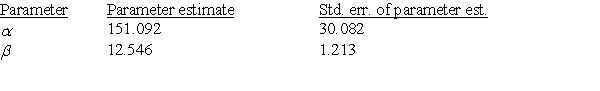A 95% confidence interval for the mean number of calories per gram of fat in sandwich menu items at fast-food restaurants is: