Exam 18: Time Series and Forecasting
Exam 1: Statistics and Data100 Questions
Exam 2: Tabular and Graphical Methods123 Questions
Exam 3: Numerical Descriptive Measures151 Questions
Exam 4: Basic Probability Concepts116 Questions
Exam 5: Discrete Probability Distributions139 Questions
Exam 6: Continuous Probability Distributions128 Questions
Exam 7: Sampling and Sampling Distributions124 Questions
Exam 8: Interval Estimation123 Questions
Exam 9: Hypothesis Testing135 Questions
Exam 10: Statistical Inference Concerning Two Populations124 Questions
Exam 11: Statistical Inference Concerning Variance111 Questions
Exam 12: Chi-Square Tests120 Questions
Exam 13: Analysis of Variance58 Questions
Exam 14: Regression Analysis140 Questions
Exam 15: Inference With Regression Models124 Questions
Exam 16: Regression Models for Nonlinear Relationships115 Questions
Exam 17: Regression Models With Dummy Variables114 Questions
Exam 18: Time Series and Forecasting124 Questions
Exam 19: Returns, Index Numbers and Inflation120 Questions
Exam 20: Nonparametric Tests108 Questions
Select questions type
Under which of the following conditions is qualitative forecasting considered attractive?
(Multiple Choice)
4.8/5  (38)
(38)
The following table shows the annual revenues (in millions of dollars)of a pharmaceutical company over the period 1990-2011. 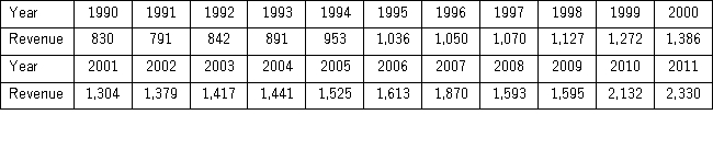 The autoregressive models of order 1 and 2,yt = β0 + β1yt - 1 + εt,and yt = β0 + β1yt - 1 + β2yt - 2 + εt,were applied on the time series to make revenue forecasts.The relevant parts of Excel regression outputs are given below.
Model AR(1):
The autoregressive models of order 1 and 2,yt = β0 + β1yt - 1 + εt,and yt = β0 + β1yt - 1 + β2yt - 2 + εt,were applied on the time series to make revenue forecasts.The relevant parts of Excel regression outputs are given below.
Model AR(1): 
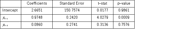
 Model AR(2):
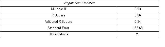
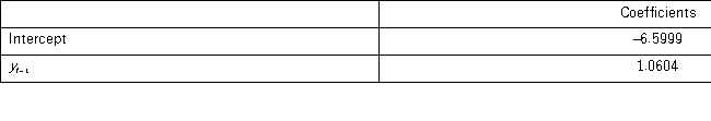
 When for AR(1),H0: β0 = 0 is tested against HA: β0 ≠ 0,the p-value of this t test shown by Excel output is 0.9590.This could suggest that the model yt = β1yt-1 + εt might be an alternative to the AR(1)model yt = β0 + β1yt-1 + εt.Excel partial output for this simplified model is as follows:
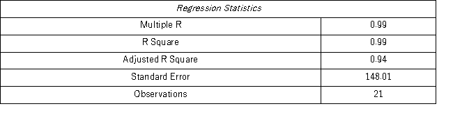
 Find the revenue forecast for 2012 through the use of yt = β1yt-1 + εt.
(Essay)
4.9/5 (36)
When the decomposition model,yt = Tt × St × It,is applied,forecasts are made as  ,where
  represents the estimated trend for seasonally adjusted time series for period t,and
  is the seasonal index for period t.
(True/False)
4.7/5 (40)
When comparing which of the following trend models is the adjusted R2 not used?
(Multiple Choice)
5.0/5 (43)
Filters
- Essay(0)
- Multiple Choice(0)
- Short Answer(0)
- True False(0)
- Matching(0)