Exam 13: Multiple Regression

SCENARIO 13-17 Given below are results from the regression analysis where the dependent variable is the number of weeks a worker is unemployed due to a layoff (Unemploy) and the independent variables are the age of the worker (Age) and a dummy variable for management position (Manager: 1 = yes, 0 = no). The results of the regression analysis are given below: Regression Statistics Multiple R 0.6391 R Square 0.4085 Adjusted R Square 0.3765 Standard Error 18.8929 Observations 40 ANOVA df SS MS F Significance F Regression 2 9119.0897 4559.5448 12.7740 0.0000 Residual 37 13206.8103 356.9408 Total 39 22325.9 Coefficients Standard Error t Stat P -value Intercept -0.2143 11.5796 -0.0185 0.9853 Age 1.4448 0.3160 4.5717 0.0000 Manager -22.5761 11.3488 -1.9893 0.0541 -Referring to SCENARIO 13-17, which of the following is the correct null hypothesis to test whether age has any effect on the number of weeks a worker is unemployed due to a layoff while holding constant the effect of the other independent variable?

SCENARIO 13-3 An economist is interested to see how consumption for an economy (in $ billions) is influenced by gross domestic product ($ billions) and aggregate price (consumer price index).The Microsoft Excel output of this regression is partially reproduced below. 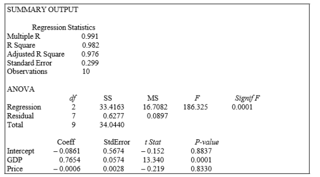-Referring to SCENARIO 13-3, one economy in the sample had an aggregate consumption level of $3 billion, a GDP of $3.5 billion, and an aggregate price level of 125.What is the residual for this data point?

SCENARIO 13-10 You worked as an intern at We Always Win Car Insurance Company last summer.You notice that individual car insurance premiums depend very much on the age of the individual and the number of traffic tickets received by the individual.You performed a regression analysis in EXCEL and obtained the following partial information: Regression Statistics Multiple R 0.8546 R Square 0.7303 Adjusted R Square 0.6853 Standard Error 226.7502 Observations 15 ANOVA df SS MS F Significance F Regression 2 835284.6500 16.2457 0.0004 Residual 12 616987.8200 Total 2287557.1200 Coefficients Standard Error t Stat P-value Lower 99\% Upper 99\% Intercept 821.2617 161.9391 5.0714 0.0003 326.6124 1315.9111 Age -1.4061 2.5988 -0.5411 0.5984 -9.3444 6.5321 Tickets 243.4401 43.2470 5.6291 0.0001 111.3406 375.5396 -Referring to SCENARIO 13-10, to test the significance of the multiple regression model, the null hypothesis should be rejected while allowing for 1% probability of committing a type I error.

SCENARIO 13-13 An econometrician is interested in evaluating the relationship of demand for building materials to mortgage rates in Los Angeles and San Francisco.He believes that the appropriate model is $Y = 10 + 5 X _ { 1 } + 8 X _ { 2 }$ where = mortgage rate in \% =1 if SF, 0 if LA Y= demand in \ 100 per capita -Referring to SCENARIO 13-13, the predicted demand in Los Angeles when the mortgage rate is 8% is .

SCENARIO 13-6 One of the most common questions of prospective house buyers pertains to the cost of heating in dollars (Y).To provide its customers with information on that matter, a large real estate firm used the following 2 variables to predict heating costs: the daily minimum outside temperature in degrees of Fahrenheit ( X1 ) and the amount of insulation in inches ( X 2 ).Given below is EXCEL output of the regression model. Regression Statistics Multiple R 0.5270 R Square 0.2778 Adjusted R Square 0.1928 Standard Error 40.9107 Observations 20 ANOVA df SS MS F Significance F Regression 2 10943.0190 5471.5095 3.2691 0.0629 Residual 17 28452.6027 1673.6825 Total 19 39395.6218 13-22 Multiple Regression Coefficients Standard Error t Stat P-volue Lower 95\% Upper 95\% Intercept 448.2925 90.7853 4.9379 0.0001 256.7522 639.8328 Temperature -2.7621 1.2371 -2.2327 0.0393 -5.3721 -0.1520 Insulation -15.9408 10.0638 -1.5840 0.1316 -37.1736 5.2919 Also SSR \mid =8343.3572 and SSR \mid =4199.2672 -Referring to SCENARIO 13-6, the partial F test forH0: Variable X1 does not significantly improve the model after variable X2 has been includedH1: Variable X1 significantly improves the model after variable X2 has been included has and degrees of freedom.

SCENARIO 13-2 A professor of industrial relations believes that an individual's wage rate at a factory (Y) depends on his performance rating (X1) and the number of economics courses the employee successfully completed in college (X2).The professor randomly selects 6 workers and collects the following information: Employee Y(\ ) 1 10 3 0 2 12 1 5 3 15 8 1 4 17 5 8 5 20 7 12 6 25 10 9 -Referring to SCENARIO 13-2, for these data, what is the estimated coefficient for performance rating, b1?

Which of the following is used to determine observations that have influential effect on the fitted model?

SCENARIO 13-19 The marketing manager for a nationally franchised lawn service company would like to study the characteristics that differentiate home owners who do and do not have a lawn service.A random sample of 30 home owners located in a suburban area near a large city was selected; 11 did not have a lawn service (code 0) and 19 had a lawn service (code 1).Additional information available concerning these 30 home owners includes family income (Income, in thousands of dollars) and lawn size (Lawn Size, in thousands of square feet). The PHStat output is given below: Binary Logistic Regression Predictor Coefficients SE Coef Z p -Value Intercept -7.8562 3.8224 -2.0553 0.0398 Income 0.0304 0.0133 2.2897 0.0220 Lawn Size 1.2804 0.6971 1.8368 0.0662 Deviance 25.3089 -Referring to SCENARIO 13-19, which of the following is the correct interpretation for theIncome slope coefficient?

SCENARIO 13-5 A microeconomist wants to determine how corporate sales are influenced by capital and wage spending by companies.She proceeds to randomly select 26 large corporations and record information in millions of dollars.The Microsoft Excel output below shows results of this multiple regression. SUMMARY OUTPUT Regression Statistics Multiple R 0.830 R Square 0.689 Adjusted R Square 0.662 Standard Error 17501.643 Observations 26 ANOVA df SS MS F Signif F Regression 2 15579777040 7789888520 25.432 0.0001 Residual 23 7045072780 306307512 Total 25 22624849820 Coeff StdError t Stat P-value Intercept 15800.0000 6038.2999 2.617 0.0154 Capital 0.1245 0.2045 0.609 0.5485 Wages 7.0762 1.4729 4.804 0.0001 -Referring to SCENARIO 13-5, what are the predicted sales (in millions of dollars) for a company spending $500 million on capital and $200 million on wages?

An interaction term in a multiple regression model may be used when the relationship between X1 and Y changes for differing values of X2.

SCENARIO 13-8 A financial analyst wanted to examine the relationship between salary (in $1,000) and 2 variables: age (X1 = Age) and experience in the field (X2 = Exper).He took a sample of 20 employees and obtained the following Microsoft Excel output: Regression Statistics Multiple R 0.8535 R Square 0.7284 Adjusted R Square 0.6964 Standard Error 10.5630 Observations 20 ANOYA df SS MS F Siqnificonce F Regression 2 5086.5764 2543.2882 22.7941 0.0000 Residual 17 1896.8050 111.5768 Total 19 6983.3814 Coefficients Standard Error t Stat P-value Lower 95\% Upper 95\% Intercept 1.5740 9.2723 0.1698 0.8672 -17.9888 21.1368 Age 1.3045 0.1956 6.6678 0.0000 0.8917 1.7173 Exper -0.1478 0.1944 -0.7604 0.4574 -0.5580 0.2624 -Referring to SCENARIO 13-8, _% of the variation in salary can be explained by the variation in experience while holding age constant.

SCENARIO 13-15 The superintendent of a school district wanted to predict the percentage of students passing a sixth- grade proficiency test.She obtained the data on percentage of students passing the proficiency test (% Passing), mean teacher salary in thousands of dollars (Salaries), and instructional spending per pupil in thousands of dollars (Spending) of 47 schools in the state. Following is the multiple regression output with Y = % Passing as the dependent variable, X1 = Salaries and X 2 = Spending: Regression Statistics Multiple R 0.4276 R Square 0.1828 Adjusted R Square 0.1457 Standard Error 5.7351 Observations 47 ANOVA df SS MS F Significance F Regression 2 323.8284 161.9142 4.9227 0.0118 Residual 44 1447.2094 32.8911 Total 46 1771.0378 Coefficients Standard Error t Stat P-value Lower 95\% Upper 95\% Intercept -72.9916 45.9106 -1.5899 0.1190 -165.5184 19.5352 Salary 2.7939 0.8974 3.1133 0.0032 0.9853 4.6025 Spending 0.3742 0.9782 0.3825 0.7039 -1.5972 2.3455 -Referring to SCENARIO 13-15, the null hypothesis should be rejected at a 5% level of significance when testing whether there is a significant relationship between percentage of students passing the proficiency test and the entire set of explanatory variables.

SCENARIO 13-17 Given below are results from the regression analysis where the dependent variable is the number of weeks a worker is unemployed due to a layoff (Unemploy) and the independent variables are the age of the worker (Age) and a dummy variable for management position (Manager: 1 = yes, 0 = no). The results of the regression analysis are given below: Regression Statistics Multiple R 0.6391 R Square 0.4085 Adjusted R Square 0.3765 Standard Error 18.8929 Observations 40 ANOVA df SS MS F Significance F Regression 2 9119.0897 4559.5448 12.7740 0.0000 Residual 37 13206.8103 356.9408 Total 39 22325.9 Coefficients Standard Error t Stat P -value Intercept -0.2143 11.5796 -0.0185 0.9853 Age 1.4448 0.3160 4.5717 0.0000 Manager -22.5761 11.3488 -1.9893 0.0541 -Referring to SCENARIO 13-17, what is the p-value of the test statistic when testing whether age has any effect on the number of weeks a worker is unemployed due to a layoff while holding constant the effect of the other independent variable?

A plot of the residuals versus an independent X shows evidence of a curvilinear effect.Which of the following statements is a possible solution?

A regression had the following results: SST = 102.55, SSE = 82.04.It can be said that 90.0% of the variation in the dependent variable is explained by the independent variables in the regression.

SCENARIO 13-15 The superintendent of a school district wanted to predict the percentage of students passing a sixth- grade proficiency test.She obtained the data on percentage of students passing the proficiency test (% Passing), mean teacher salary in thousands of dollars (Salaries), and instructional spending per pupil in thousands of dollars (Spending) of 47 schools in the state. Following is the multiple regression output with Y = % Passing as the dependent variable, X1 = Salaries and X 2 = Spending: Regression Statistics Multiple R 0.4276 R Square 0.1828 Adjusted R Square 0.1457 Standard Error 5.7351 Observations 47 ANOVA df SS MS F Significance F Regression 2 323.8284 161.9142 4.9227 0.0118 Residual 44 1447.2094 32.8911 Total 46 1771.0378 Coefficients Standard Error t Stat P-value Lower 95\% Upper 95\% Intercept -72.9916 45.9106 -1.5899 0.1190 -165.5184 19.5352 Salary 2.7939 0.8974 3.1133 0.0032 0.9853 4.6025 Spending 0.3742 0.9782 0.3825 0.7039 -1.5972 2.3455 -Referring to SCENARIO 13-15, the alternative hypothesis H 1 :At least one of $\beta$ j $\neq$ 0 for j =1, 2 implies that percentage of students passing the proficiency test is related to both of the explanatory variables.

SCENARIO 13-8 A financial analyst wanted to examine the relationship between salary (in $1,000) and 2 variables: age (X1 = Age) and experience in the field (X2 = Exper).He took a sample of 20 employees and obtained the following Microsoft Excel output: Regression Statistics Multiple R 0.8535 R Square 0.7284 Adjusted R Square 0.6964 Standard Error 10.5630 Observations 20 ANOYA df SS MS F Siqnificonce F Regression 2 5086.5764 2543.2882 22.7941 0.0000 Residual 17 1896.8050 111.5768 Total 19 6983.3814 Coefficients Standard Error t Stat P-value Lower 95\% Upper 95\% Intercept 1.5740 9.2723 0.1698 0.8672 -17.9888 21.1368 Age 1.3045 0.1956 6.6678 0.0000 0.8917 1.7173 Exper -0.1478 0.1944 -0.7604 0.4574 -0.5580 0.2624 -Referring to SCENARIO 13-8, the analyst wants to use an F-test to test H0 : $\beta$ 1 = $\beta$ 2 = 0 .The appropriate alternative hypothesis is _.

In calculating the standard error of the estimate, SYX =MSE , there are n - k - 1 degrees of freedom, where n is the sample size and k represents the number of independent variables in the model.

SCENARIO 13-10 You worked as an intern at We Always Win Car Insurance Company last summer.You notice that individual car insurance premiums depend very much on the age of the individual and the number of traffic tickets received by the individual.You performed a regression analysis in EXCEL and obtained the following partial information: Regression Statistics Multiple R 0.8546 R Square 0.7303 Adjusted R Square 0.6853 Standard Error 226.7502 Observations 15 ANOVA df SS MS F Significance F Regression 2 835284.6500 16.2457 0.0004 Residual 12 616987.8200 Total 2287557.1200 Coefficients Standard Error t Stat P-value Lower 99\% Upper 99\% Intercept 821.2617 161.9391 5.0714 0.0003 326.6124 1315.9111 Age -1.4061 2.5988 -0.5411 0.5984 -9.3444 6.5321 Tickets 243.4401 43.2470 5.6291 0.0001 111.3406 375.5396 -Referring to SCENARIO 13-10, the regression sum of squares that is missing in the ANOVAtable should be .

SCENARIO 13-10 You worked as an intern at We Always Win Car Insurance Company last summer.You notice that individual car insurance premiums depend very much on the age of the individual and the number of traffic tickets received by the individual.You performed a regression analysis in EXCEL and obtained the following partial information: Regression Statistics Multiple R 0.8546 R Square 0.7303 Adjusted R Square 0.6853 Standard Error 226.7502 Observations 15 ANOVA df SS MS F Significance F Regression 2 835284.6500 16.2457 0.0004 Residual 12 616987.8200 Total 2287557.1200 Coefficients Standard Error t Stat P-value Lower 99\% Upper 99\% Intercept 821.2617 161.9391 5.0714 0.0003 326.6124 1315.9111 Age -1.4061 2.5988 -0.5411 0.5984 -9.3444 6.5321 Tickets 243.4401 43.2470 5.6291 0.0001 111.3406 375.5396 -Referring to SCENARIO 13-10, to test the significance of the multiple regression model, the p- value of the test statistic in the sample is .