SCENARIO 13-10 You worked as an intern at We Always Win Car Insurance Company last summer.You notice that individual car insurance premiums depend very much on the age of the individual and the number of traffic tickets received by the individual.You performed a regression analysis in EXCEL and obtained the following partial information: \[\begin{array}{l} \begin{array} { l r } \hline { \text { Regression Statistics } } \\ \hline \text { Multiple R } & 0.8546 \\ \text { R Square } & 0.7303 \\ \text { Adjusted R Square } & 0.6853 \\ \text { Standard Error } & 226.7502 \\ \text { Observations } & 15 \\ \hline \end{array}\\\\ \text { ANOVA }\\ \begin{array}{lrrrrrr} & d f & & \text { SS } & \text { MS } & \text { F } & \text { Significance } F \\ \hline \text { Regression } & & 2 & & \text { 835284.6500 } & 16.2457 & 0.0004 \\ \text { Residual } & & 12 & 616987.8200 & & & \\ \text { Total } & & & 2287557.1200 & & & \\ \hline \end{array}\\\\ \begin{array} { l r r r r r r } \hline & \text { Coefficients } & \text { Standard Error } & { t \text { Stat } } & \text { P-value } & \text { Lower 99\% } & { \text { Upper 99\% } } \\ \hline \text { Intercept } & 821.2617 & 161.9391 & 5.0714 & 0.0003 & 326.6124 & 1315.9111 \\ \text { Age } & - 1.4061 & 2.5988 & - 0.5411 & 0.5984 & - 9.3444 & 6.5321 \\ \text { Tickets } & 243.4401 & 43.2470 & 5.6291 & 0.0001 & 111.3406 & 375.5396 \\ \hline \end{array} \end{array}\] -Referring to SCENARIO 13-10, the proportion of the total variability in insurance premiums that can be explained by AGE and TICKETS is .

The answer of SCENARIO 13-10 You worked as an intern at...

SCENARIO 13-7 The department head of the accounting department wanted to see if she could predict the GPA of students using the number of course units and total SAT scores of each.She takes a sample of 6 students and generates the following Microsoft Excel output: SUMMARY OUTPUT Regression Statistics $\begin{array} { l l } \text { Multiple R } & 0.916 \\ \text { R Square } & 0.839 \\ \text { Adjusted R Square } & 0.732 \\ \text { Standard Error } & 0.24685 \\ \text { Observations } & 6 \end{array}$ ANOVA $\begin{array} { l r c c r c } & d f & \text { SS } & \text { MS } & F & \text { Signif } F \\ \text { Regression } & 2 & 0.95219 & 0.47610 & 7.813 & 0.0646 \\ \text { Residual } & 3 & 0.18281 & 0.06094 & & \\ \text { Total } & 5 & 1.13500 & & & \end{array}$ $\begin{array} { l c r c c } & \text { Coeff } & \text { StdError } & t \text { Stat } & P \text {-value } \\ \text { Intercept } & 4.593897 & 1.13374542 & 4.052 & 0.0271 \\ \text { Units } & - 0.247270 & 0.06268485 & - 3.945 & 0.0290 \\ \text { Total SAT } & 0.001443 & 0.00101241 & 1.425 & 0.2494 \end{array}$ -Referring to SCENARIO 13-7, the department head wants to use a t test to test for the significance of the coefficient of X1.The p-value of the test is .

The answer of SCENARIO 13-7 The department head of the accounting...

SCENARIO 13-11 A weight-loss clinic wants to use regression analysis to build a model for weight loss of a client (measured in pounds).Two variables thought to affect weight loss are client's length of time on the weight-loss program and time of session.These variables are described below: Y = Weight loss (in pounds) X1 = Length of time in weight-loss program (in months) X2 = 1 if morning session, 0 if not Data for 25 clients on a weight-loss program at the clinic were collected and used to fit the interaction model: \[Y = \beta _ { 0 } + \beta _ { 1 } X _ { 1 } + \beta _ { 2 } X _ { 2 } + \beta _ { 3 } X _ { 1 } X _ { 2 } + \varepsilon\] Output from Microsoft Excel follows: $\begin{array}{lr} {\text { Regression Statistics }} \\ \hline \text { Multiple R } & 0.7308 \\ \text { R Square } & 0.5341 \\ \text { Adjusted R Square } & 0.4675 \\ \text { Standard Error } & 43.3275 \\ \text { Observations } & 25\\ \hline \end{array}$ $\text { ANOVA }$ $\begin{array}{lrrrrr} \hline&\text { df } & \text { SS }&M S &F & \text { Significance } F\\ \hline\text { Regression } & 3 & 45194.0661 & 15064.6887 & 8.0248 & 0.0009 \\ \text { Residual } & 21 & 39422.6542 & 1877.2692 & & \\ \text { Total } & 24 & 84616.7203 & &\\ \hline \end{array}$ $\begin{array}{lrrrrrr} \hline & \text { Coefficients } & \text { Standard Error } &{\text { t Stat }} & \text { P-value } & \text { Lower 99\% } & \text { Upper 99\% } \\ \hline \text { Intercept } & -20.7298 & 22.3710 & -0.9266 & 0.3646 & -84.0702 & 42.6106 \\ \text { Length } & 7.2472 & 1.4992 & 4.8340 & 0.0001 & 3.0024 & 11.4919 \\ \text { Morn } & 90.1981 & 40.2336 & 2.2419 & 0.0359 & -23.7176 & 204.1138 \\ \text { Length x Morn } & -5.1024 & 3.3511 & -1.5226 & 0.1428 & -14.5905 & 4.3857 \\ \hline \end{array}$ -In a multiple regression model, the adjusted r 2

A) cannot be negative. B) can sometimes be negative. C) can sometimes be greater than +1. D) has to fall between 0 and +1. A) cannot be negative. B) can sometimes be negative. C) can sometimes be greater than +1. D) has to fall between 0 and +1.

SCENARIO 13-4 A real estate builder wishes to determine how house size (House) is influenced by family income (Income) and family size (Size).House size is measured in hundreds of square feet and income is measured in thousands of dollars.The builder randomly selected 50 families and ran the multiple regression.Partial Microsoft Excel output is provided below: $\begin{array}{lr} \hline{\text { Regression Statistics }} \\ \hline \text { Multiple R } & 0.8479 \\ \text { R Square } & 0.7189 \\ \text { Adjusted R Square } & 0.7069 \\ \text { Standard Error } & 17.5571 \\ \text { Observations } & 50\\ \hline \end{array}$ $\text { ANOVA }$ $\begin{array}{lrrrrr} & d f & \text { SS } & {M S} & F & \text { Significance } F \\ \hline \text { Regression } & & & 37043.3236 & 18521.6618 & 0.0000 \\ \text { Residual } & & 14487.7627 & 308.2503 & \\ \text { Total } & & 49 & 51531.0863 & & \end{array}$ $\begin{array}{lrrrr} \hline & \text { Coefficients } & \text { Standard Error } &{t \text { Stat }} & \text { P-value } \\ \hline \text { Intercept } & -5.5146 & 7.2273 & -0.7630 & 0.4493 \\ \text { Income } & 0.4262 & 0.0392 & 10.8668 & 0.0000 \\ \text { Size } & 5.5437 & 1.6949 & 3.2708 & 0.0020\\ \hline \end{array}$ $\text { Also } \operatorname{SSR}\left(X_{1} \mid X_{2}\right)=36400.6326 \text { and } \operatorname{SSR}\left(X_{2} \mid X_{1}\right)=3297.7917$ -Referring to SCENARIO 13-4, at the 0.01 level of significance, what conclusion should the builder draw regarding the inclusion of Size in the regression model?

A) Size is significant in explaining house size and should be included in the model because its p-value is less than 0.01. B) Size is significant in explaining house size and should be included in the model because its p-value is more than 0.01. C) Size is not significant in explaining house size and should not be included in the model because its p-value is less than 0.01. D) Size is not significant in explaining house size and should not be included in the model because its p-value is more than 0.01. A) Size is significant in explaining house size and should be included in the model because its p-value is less than 0.01. B) Size is significant in explaining house size and should be included in the model because its p-value is more than 0.01. C) Size is not significant in explaining house size and should not be included in the model because its p-value is less than 0.01. D) Size is not significant in explaining house size and should not be included in the model because its p-value is more than 0.01.

SCENARIO 13-10 You worked as an intern at We Always Win Car Insurance Company last summer.You notice that individual car insurance premiums depend very much on the age of the individual and the number of traffic tickets received by the individual.You performed a regression analysis in EXCEL and obtained the following partial information: \[\begin{array}{l} \begin{array} { l r } \hline { \text { Regression Statistics } } \\ \hline \text { Multiple R } & 0.8546 \\ \text { R Square } & 0.7303 \\ \text { Adjusted R Square } & 0.6853 \\ \text { Standard Error } & 226.7502 \\ \text { Observations } & 15 \\ \hline \end{array}\\\\ \text { ANOVA }\\ \begin{array}{lrrrrrr} & d f & & \text { SS } & \text { MS } & \text { F } & \text { Significance } F \\ \hline \text { Regression } & & 2 & & \text { 835284.6500 } & 16.2457 & 0.0004 \\ \text { Residual } & & 12 & 616987.8200 & & & \\ \text { Total } & & & 2287557.1200 & & & \\ \hline \end{array}\\\\ \begin{array} { l r r r r r r } \hline & \text { Coefficients } & \text { Standard Error } & { t \text { Stat } } & \text { P-value } & \text { Lower 99\% } & { \text { Upper 99\% } } \\ \hline \text { Intercept } & 821.2617 & 161.9391 & 5.0714 & 0.0003 & 326.6124 & 1315.9111 \\ \text { Age } & - 1.4061 & 2.5988 & - 0.5411 & 0.5984 & - 9.3444 & 6.5321 \\ \text { Tickets } & 243.4401 & 43.2470 & 5.6291 & 0.0001 & 111.3406 & 375.5396 \\ \hline \end{array} \end{array}\] -Referring to SCENARIO 13-10, the residual mean squares (MSE) that are missing in theANOVA table should be .

The answer of SCENARIO 13-10 You worked as an intern at...

SCENARIO 13-2 A professor of industrial relations believes that an individual's wage rate at a factory (Y) depends on his performance rating (X1) and the number of economics courses the employee successfully completed in college (X2).The professor randomly selects 6 workers and collects the following information: \[\begin{array} { c c r r } \text { Employee } & Y ( \$ ) & \underline { X } _ { 1 } & X _ { 2 } \\ 1 & 10 & 3 & 0 \\ 2 & 12 & 1 & 5 \\ 3 & 15 & 8 & 1 \\ 4 & 17 & 5 & 8 \\ 5 & 20 & 7 & 12 \\ 6 & 25 & 10 & 9 \end{array}\] -Referring to SCENARIO 13-2, suppose an employee had never taken an economics course and managed to score a 5 on his performance rating.What is his estimated expected wage rate?

A) 10.90 B) 12.20 C) 17.23 D) 25.11 A) 10.90 B) 12.20 C) 17.23 D) 25.11

SCENARIO 13-7 The department head of the accounting department wanted to see if she could predict the GPA of students using the number of course units and total SAT scores of each.She takes a sample of 6 students and generates the following Microsoft Excel output: SUMMARY OUTPUT Regression Statistics $\begin{array} { l l } \text { Multiple R } & 0.916 \\ \text { R Square } & 0.839 \\ \text { Adjusted R Square } & 0.732 \\ \text { Standard Error } & 0.24685 \\ \text { Observations } & 6 \end{array}$ ANOVA $\begin{array} { l r c c r c } & d f & \text { SS } & \text { MS } & F & \text { Signif } F \\ \text { Regression } & 2 & 0.95219 & 0.47610 & 7.813 & 0.0646 \\ \text { Residual } & 3 & 0.18281 & 0.06094 & & \\ \text { Total } & 5 & 1.13500 & & & \end{array}$ $\begin{array} { l c r c c } & \text { Coeff } & \text { StdError } & t \text { Stat } & P \text {-value } \\ \text { Intercept } & 4.593897 & 1.13374542 & 4.052 & 0.0271 \\ \text { Units } & - 0.247270 & 0.06268485 & - 3.945 & 0.0290 \\ \text { Total SAT } & 0.001443 & 0.00101241 & 1.425 & 0.2494 \end{array}$ -Referring to SCENARIO 13-7, the net regression coefficient of X2 is .

The answer of SCENARIO 13-7 The department head of the accounting...

SCENARIO 13-4 A real estate builder wishes to determine how house size (House) is influenced by family income (Income) and family size (Size).House size is measured in hundreds of square feet and income is measured in thousands of dollars.The builder randomly selected 50 families and ran the multiple regression.Partial Microsoft Excel output is provided below: $\begin{array}{lr} \hline{\text { Regression Statistics }} \\ \hline \text { Multiple R } & 0.8479 \\ \text { R Square } & 0.7189 \\ \text { Adjusted R Square } & 0.7069 \\ \text { Standard Error } & 17.5571 \\ \text { Observations } & 50\\ \hline \end{array}$ $\text { ANOVA }$ $\begin{array}{lrrrrr} & d f & \text { SS } & {M S} & F & \text { Significance } F \\ \hline \text { Regression } & & & 37043.3236 & 18521.6618 & 0.0000 \\ \text { Residual } & & 14487.7627 & 308.2503 & \\ \text { Total } & & 49 & 51531.0863 & & \end{array}$ $\begin{array}{lrrrr} \hline & \text { Coefficients } & \text { Standard Error } &{t \text { Stat }} & \text { P-value } \\ \hline \text { Intercept } & -5.5146 & 7.2273 & -0.7630 & 0.4493 \\ \text { Income } & 0.4262 & 0.0392 & 10.8668 & 0.0000 \\ \text { Size } & 5.5437 & 1.6949 & 3.2708 & 0.0020\\ \hline \end{array}$ $\text { Also } \operatorname{SSR}\left(X_{1} \mid X_{2}\right)=36400.6326 \text { and } \operatorname{SSR}\left(X_{2} \mid X_{1}\right)=3297.7917$ -Referring to SCENARIO 13-4, what are the regression degrees of freedom that are missing from the output?

A) 2 B) 47 C) 49 D) 50 A) 2 B) 47 C) 49 D) 50

SCENARIO 13-17 Given below are results from the regression analysis where the dependent variable is the number of weeks a worker is unemployed due to a layoff (Unemploy) and the independent variables are the age of the worker (Age) and a dummy variable for management position (Manager: 1 = yes, 0 = no). The results of the regression analysis are given below: \[\begin{array}{l} \begin{array} { l r } \hline { \text { Regression Statistics } } \\ \hline \text { Multiple R } & 0.6391 \\ \text { R Square } & 0.4085 \\ \text { Adjusted R Square } & 0.3765 \\ \text { Standard Error } & 18.8929 \\ \text { Observations } & 40 \\ \hline \end{array}\\\\ \text { ANOVA }\\ \begin{array} { l r r r r r } \hline &{ \text { df } } & { \text { SS } } & { \text { MS } } &{ \text { F } } & { \text { Significance } F } \\ \hline \text { Regression } & 2 & 9119.0897 & 4559.5448 & 12.7740 & 0.0000 \\ \text { Residual } & 37 & 13206.8103 & 356.9408 & \\ \text { Total } & 39 & 22325.9 & & \\ \hline \end{array}\\\\ \begin{array} { l r r r r } \hline & \text { Coefficients } & \text { Standard Error } & { t \text { Stat } } & { P \text {-value } } \\ \hline \text { Intercept } & - 0.2143 & 11.5796 & - 0.0185 & 0.9853 \\ \text { Age } & 1.4448 & 0.3160 & 4.5717 & 0.0000 \\ \text { Manager } & - 22.5761 & 11.3488 & - 1.9893 & 0.0541 \\ \hline \end{array} \end{array}\] -Referring to SCENARIO 13-17, predict the number of weeks being unemployed due to a layoff for a worker who is a thirty-year old and is a manager.

The answer of SCENARIO 13-17 Given below are results from the...

SCENARIO 13-17 Given below are results from the regression analysis where the dependent variable is the number of weeks a worker is unemployed due to a layoff (Unemploy) and the independent variables are the age of the worker (Age) and a dummy variable for management position (Manager: 1 = yes, 0 = no). The results of the regression analysis are given below: \[\begin{array}{l} \begin{array} { l r } \hline { \text { Regression Statistics } } \\ \hline \text { Multiple R } & 0.6391 \\ \text { R Square } & 0.4085 \\ \text { Adjusted R Square } & 0.3765 \\ \text { Standard Error } & 18.8929 \\ \text { Observations } & 40 \\ \hline \end{array}\\\\ \text { ANOVA }\\ \begin{array} { l r r r r r } \hline &{ \text { df } } & { \text { SS } } & { \text { MS } } &{ \text { F } } & { \text { Significance } F } \\ \hline \text { Regression } & 2 & 9119.0897 & 4559.5448 & 12.7740 & 0.0000 \\ \text { Residual } & 37 & 13206.8103 & 356.9408 & \\ \text { Total } & 39 & 22325.9 & & \\ \hline \end{array}\\\\ \begin{array} { l r r r r } \hline & \text { Coefficients } & \text { Standard Error } & { t \text { Stat } } & { P \text {-value } } \\ \hline \text { Intercept } & - 0.2143 & 11.5796 & - 0.0185 & 0.9853 \\ \text { Age } & 1.4448 & 0.3160 & 4.5717 & 0.0000 \\ \text { Manager } & - 22.5761 & 11.3488 & - 1.9893 & 0.0541 \\ \hline \end{array} \end{array}\] -Referring to SCENARIO 13-17, what is the value of the test statistic to determine whether there is a significant relationship between the number of weeks a worker is unemployed due to a layoff and the entire set of explanatory variables?

The answer of SCENARIO 13-17 Given below are results from the...

Exam 13: Multiple Regression

SCENARIO 13-7 The department head of the accounting department wanted to see if she could predict the GPA of students using the number of course units and total SAT scores of each.She takes a sample of 6 students and generates the following Microsoft Excel output: SUMMARY OUTPUT Regression Statistics Multiple R 0.916 R Square 0.839 Adjusted R Square 0.732 Standard Error 0.24685 Observations 6 ANOVA df SS MS F Signif F Regression 2 0.95219 0.47610 7.813 0.0646 Residual 3 0.18281 0.06094 Total 5 1.13500 Coeff StdError t Stat P -value Intercept 4.593897 1.13374542 4.052 0.0271 Units -0.247270 0.06268485 -3.945 0.0290 Total SAT 0.001443 0.00101241 1.425 0.2494 -Referring to SCENARIO 13-7, the department head wants to test H0: $\beta$ 1 = $\beta$ 2 = 0 .At a level of significance of 0.05, the null hypothesis is rejected.

(True/False)

4.8/5

(41)

Question 161

SCENARIO 13-10 You worked as an intern at We Always Win Car Insurance Company last summer.You notice that individual car insurance premiums depend very much on the age of the individual and the number of traffic tickets received by the individual.You performed a regression analysis in EXCEL and obtained the following partial information: Regression Statistics Multiple R 0.8546 R Square 0.7303 Adjusted R Square 0.6853 Standard Error 226.7502 Observations 15 ANOVA df SS MS F Significance F Regression 2 835284.6500 16.2457 0.0004 Residual 12 616987.8200 Total 2287557.1200 Coefficients Standard Error t Stat P-value Lower 99\% Upper 99\% Intercept 821.2617 161.9391 5.0714 0.0003 326.6124 1315.9111 Age -1.4061 2.5988 -0.5411 0.5984 -9.3444 6.5321 Tickets 243.4401 43.2470 5.6291 0.0001 111.3406 375.5396 -Referring to SCENARIO 13-10, the proportion of the total variability in insurance premiums that can be explained by AGE and TICKETS is .

(Short Answer)

4.9/5

(42)

Question 162

When an additional explanatory variable is introduced into a multiple regression model, the coefficient of multiple determination will never decrease.

(True/False)

4.9/5

(33)

Question 163

SCENARIO 13-7 The department head of the accounting department wanted to see if she could predict the GPA of students using the number of course units and total SAT scores of each.She takes a sample of 6 students and generates the following Microsoft Excel output: SUMMARY OUTPUT Regression Statistics Multiple R 0.916 R Square 0.839 Adjusted R Square 0.732 Standard Error 0.24685 Observations 6 ANOVA df SS MS F Signif F Regression 2 0.95219 0.47610 7.813 0.0646 Residual 3 0.18281 0.06094 Total 5 1.13500 Coeff StdError t Stat P -value Intercept 4.593897 1.13374542 4.052 0.0271 Units -0.247270 0.06268485 -3.945 0.0290 Total SAT 0.001443 0.00101241 1.425 0.2494 -Referring to SCENARIO 13-7, the department head wants to use a t test to test for the significance of the coefficient of X1.The p-value of the test is .

(Short Answer)

4.9/5

(36)

Question 164

SCENARIO 13-11 A weight-loss clinic wants to use regression analysis to build a model for weight loss of a client (measured in pounds).Two variables thought to affect weight loss are client's length of time on the weight-loss program and time of session.These variables are described below: Y = Weight loss (in pounds) X1 = Length of time in weight-loss program (in months) X2 = 1 if morning session, 0 if not Data for 25 clients on a weight-loss program at the clinic were collected and used to fit the interaction model: $Y = \beta _ { 0 } + \beta _ { 1 } X _ { 1 } + \beta _ { 2 } X _ { 2 } + \beta _ { 3 } X _ { 1 } X _ { 2 } + \varepsilon$ Output from Microsoft Excel follows: Regression Statistics Multiple R 0.7308 R Square 0.5341 Adjusted R Square 0.4675 Standard Error 43.3275 Observations 25 $\text { ANOVA }$ df SS MS F Significance F Regression 3 45194.0661 15064.6887 8.0248 0.0009 Residual 21 39422.6542 1877.2692 Total 24 84616.7203 Coefficients Standard Error t Stat P-value Lower 99\% Upper 99\% Intercept -20.7298 22.3710 -0.9266 0.3646 -84.0702 42.6106 Length 7.2472 1.4992 4.8340 0.0001 3.0024 11.4919 Morn 90.1981 40.2336 2.2419 0.0359 -23.7176 204.1138 Length x Morn -5.1024 3.3511 -1.5226 0.1428 -14.5905 4.3857 -In a multiple regression model, the adjusted r 2

(Multiple Choice)

4.8/5

(32)

Question 165

SCENARIO 13-18 A logistic regression model was estimated in order to predict the probability that a randomly chosen university or college would be a private university using information on mean total Scholastic Aptitude Test score (SAT) at the university or college and whether the TOEFL criterion is at least 90 (Toefl90 = 1 if yes, 0 otherwise.) The dependent variable, Y, is school type (Type = 1 if private and 0 otherwise).There are 80 universities in the sample. The PHStat output is given below: Binary Logistic Regression Predictor Coefficients SE Coef Z p -Value Intercept -3.9594 1.6741 -2.3650 0.0180 SAT 0.0028 0.0011 2.5459 0.0109 Toefl90:1 0.1928 0.5827 0.3309 0.7407 Deviance 101.9826 -Referring to SCENARIO 13-18, there is not enough evidence to conclude that Toefl90 makes a significant contribution to the model in the presence of SAT at a 0.05 level of significance.

(True/False)

4.8/5

(30)

Question 166

SCENARIO 13-9 You decide to predict gasoline prices in different cities and towns in the United States for your term project.Your dependent variable is price of gasoline per gallon and your explanatory variables are per capita income and the number of firms that manufacture automobile parts in and around the city.You collected data of 32 cities and obtained a regression sum of squares SSR= 122.8821.Your computed value of standard error of the estimate is 1.9549. -Referring to SCENARIO 13-9, what is the value of the coefficient of multiple determination?

(Short Answer)

4.8/5

(35)

Question 167

SCENARIO 13-4 A real estate builder wishes to determine how house size (House) is influenced by family income (Income) and family size (Size).House size is measured in hundreds of square feet and income is measured in thousands of dollars.The builder randomly selected 50 families and ran the multiple regression.Partial Microsoft Excel output is provided below: Regression Statistics Multiple R 0.8479 R Square 0.7189 Adjusted R Square 0.7069 Standard Error 17.5571 Observations 50 $\text { ANOVA }$ df SS MS F Significance F Regression 37043.3236 18521.6618 0.0000 Residual 14487.7627 308.2503 Total 49 51531.0863 Coefficients Standard Error t Stat P-value Intercept -5.5146 7.2273 -0.7630 0.4493 Income 0.4262 0.0392 10.8668 0.0000 Size 5.5437 1.6949 3.2708 0.0020 $\text { Also } \operatorname{SSR}\left(X_{1} \mid X_{2}\right)=36400.6326 \text { and } \operatorname{SSR}\left(X_{2} \mid X_{1}\right)=3297.7917$ -Referring to SCENARIO 13-4, at the 0.01 level of significance, what conclusion should the builder draw regarding the inclusion of Size in the regression model?

(Multiple Choice)

4.8/5

(36)

Question 168

SCENARIO 13-10 You worked as an intern at We Always Win Car Insurance Company last summer.You notice that individual car insurance premiums depend very much on the age of the individual and the number of traffic tickets received by the individual.You performed a regression analysis in EXCEL and obtained the following partial information: Regression Statistics Multiple R 0.8546 R Square 0.7303 Adjusted R Square 0.6853 Standard Error 226.7502 Observations 15 ANOVA df SS MS F Significance F Regression 2 835284.6500 16.2457 0.0004 Residual 12 616987.8200 Total 2287557.1200 Coefficients Standard Error t Stat P-value Lower 99\% Upper 99\% Intercept 821.2617 161.9391 5.0714 0.0003 326.6124 1315.9111 Age -1.4061 2.5988 -0.5411 0.5984 -9.3444 6.5321 Tickets 243.4401 43.2470 5.6291 0.0001 111.3406 375.5396 -Referring to SCENARIO 13-10, the residual mean squares (MSE) that are missing in theANOVA table should be .

(Short Answer)

4.8/5

(30)

Question 169

SCENARIO 13-3 An economist is interested to see how consumption for an economy (in $ billions) is influenced by gross domestic product ($ billions) and aggregate price (consumer price index).The Microsoft Excel output of this regression is partially reproduced below. 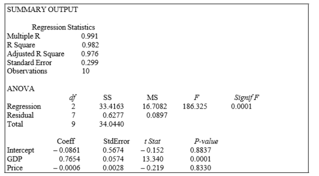-Referring to SCENARIO 13-3, one economy in the sample had an aggregate consumption level of $4 billion, a GDP of $6 billion, and an aggregate price level of 200.What is the residual for this data point?

(Multiple Choice)

4.8/5

(28)

Question 170

SCENARIO 13-19 The marketing manager for a nationally franchised lawn service company would like to study the characteristics that differentiate home owners who do and do not have a lawn service.A random sample of 30 home owners located in a suburban area near a large city was selected; 11 did not have a lawn service (code 0) and 19 had a lawn service (code 1).Additional information available concerning these 30 home owners includes family income (Income, in thousands of dollars) and lawn size (Lawn Size, in thousands of square feet). The PHStat output is given below: Binary Logistic Regression Predictor Coefficients SE Coef Z p -Value Intercept -7.8562 3.8224 -2.0553 0.0398 Income 0.0304 0.0133 2.2897 0.0220 Lawn Size 1.2804 0.6971 1.8368 0.0662 Deviance 25.3089 -Referring to SCENARIO 13-19, what is the p-value of the test statistic when testing whetherLawnSize makes a significant contribution to the model in the presence of Income?

(Short Answer)

4.9/5

(30)

Question 171

SCENARIO 13-2 A professor of industrial relations believes that an individual's wage rate at a factory (Y) depends on his performance rating (X1) and the number of economics courses the employee successfully completed in college (X2).The professor randomly selects 6 workers and collects the following information: Employee Y(\ ) 1 10 3 0 2 12 1 5 3 15 8 1 4 17 5 8 5 20 7 12 6 25 10 9 -Referring to SCENARIO 13-2, suppose an employee had never taken an economics course and managed to score a 5 on his performance rating.What is his estimated expected wage rate?

(Multiple Choice)

4.8/5

(32)

Question 172

SCENARIO 13-15 The superintendent of a school district wanted to predict the percentage of students passing a sixth- grade proficiency test.She obtained the data on percentage of students passing the proficiency test (% Passing), mean teacher salary in thousands of dollars (Salaries), and instructional spending per pupil in thousands of dollars (Spending) of 47 schools in the state. Following is the multiple regression output with Y = % Passing as the dependent variable, X1 = Salaries and X 2 = Spending: Regression Statistics Multiple R 0.4276 R Square 0.1828 Adjusted R Square 0.1457 Standard Error 5.7351 Observations 47 ANOVA df SS MS F Significance F Regression 2 323.8284 161.9142 4.9227 0.0118 Residual 44 1447.2094 32.8911 Total 46 1771.0378 Coefficients Standard Error t Stat P-value Lower 95\% Upper 95\% Intercept -72.9916 45.9106 -1.5899 0.1190 -165.5184 19.5352 Salary 2.7939 0.8974 3.1133 0.0032 0.9853 4.6025 Spending 0.3742 0.9782 0.3825 0.7039 -1.5972 2.3455 -Referring to SCENARIO 13-15, the null hypothesis H0 : $\beta$ 1 = $\beta$ 2 = 0 implies that percentage of students passing the proficiency test is not related to one of the explanatory variables.

(True/False)

4.9/5

(31)

Question 173

SCENARIO 13-7 The department head of the accounting department wanted to see if she could predict the GPA of students using the number of course units and total SAT scores of each.She takes a sample of 6 students and generates the following Microsoft Excel output: SUMMARY OUTPUT Regression Statistics Multiple R 0.916 R Square 0.839 Adjusted R Square 0.732 Standard Error 0.24685 Observations 6 ANOVA df SS MS F Signif F Regression 2 0.95219 0.47610 7.813 0.0646 Residual 3 0.18281 0.06094 Total 5 1.13500 Coeff StdError t Stat P -value Intercept 4.593897 1.13374542 4.052 0.0271 Units -0.247270 0.06268485 -3.945 0.0290 Total SAT 0.001443 0.00101241 1.425 0.2494 -Referring to SCENARIO 13-7, the net regression coefficient of X2 is .

(Short Answer)

4.8/5

(32)

Question 174

SCENARIO 13-19 The marketing manager for a nationally franchised lawn service company would like to study the characteristics that differentiate home owners who do and do not have a lawn service.A random sample of 30 home owners located in a suburban area near a large city was selected; 11 did not have a lawn service (code 0) and 19 had a lawn service (code 1).Additional information available concerning these 30 home owners includes family income (Income, in thousands of dollars) and lawn size (Lawn Size, in thousands of square feet). The PHStat output is given below: Binary Logistic Regression Predictor Coefficients SE Coef Z p -Value Intercept -7.8562 3.8224 -2.0553 0.0398 Income 0.0304 0.0133 2.2897 0.0220 Lawn Size 1.2804 0.6971 1.8368 0.0662 Deviance 25.3089 -Referring to SCENARIO 13-19, what is the estimated probability that a home owner with a family income of $50,000 and a lawn size of 2,000 square feet will purchase a lawn service?

(Short Answer)

4.8/5

(41)

Question 175

SCENARIO 13-19 The marketing manager for a nationally franchised lawn service company would like to study the characteristics that differentiate home owners who do and do not have a lawn service.A random sample of 30 home owners located in a suburban area near a large city was selected; 11 did not have a lawn service (code 0) and 19 had a lawn service (code 1).Additional information available concerning these 30 home owners includes family income (Income, in thousands of dollars) and lawn size (Lawn Size, in thousands of square feet). The PHStat output is given below: Binary Logistic Regression Predictor Coefficients SE Coef Z p -Value Intercept -7.8562 3.8224 -2.0553 0.0398 Income 0.0304 0.0133 2.2897 0.0220 Lawn Size 1.2804 0.6971 1.8368 0.0662 Deviance 25.3089 -Referring to SCENARIO 13-19, what is the estimated probability that a home owner with a family income of $100,000 and a lawn size of 5,000 square feet will purchase a lawn service?

(Short Answer)

4.7/5

(39)

Question 176

SCENARIO 13-14 An automotive engineer would like to be able to predict automobile mileages.She believes that the two most important characteristics that affect mileage are horsepower and the number of cylinders (4 or 6) of a car.She believes that the appropriate model is Y = 40 - 0.05X1 + 20X2 - 0.1X1X2 where X1 = horsepower X2 = 1 if 4 cylinders, 0 if 6 cylinders Y = mileage. -Referring to SCENARIO 13-14, the predicted mileage for a 200 horsepower, 4-cylinder car is_.

(Short Answer)

4.8/5

(34)

Question 177

SCENARIO 13-4 A real estate builder wishes to determine how house size (House) is influenced by family income (Income) and family size (Size).House size is measured in hundreds of square feet and income is measured in thousands of dollars.The builder randomly selected 50 families and ran the multiple regression.Partial Microsoft Excel output is provided below: Regression Statistics Multiple R 0.8479 R Square 0.7189 Adjusted R Square 0.7069 Standard Error 17.5571 Observations 50 $\text { ANOVA }$ df SS MS F Significance F Regression 37043.3236 18521.6618 0.0000 Residual 14487.7627 308.2503 Total 49 51531.0863 Coefficients Standard Error t Stat P-value Intercept -5.5146 7.2273 -0.7630 0.4493 Income 0.4262 0.0392 10.8668 0.0000 Size 5.5437 1.6949 3.2708 0.0020 $\text { Also } \operatorname{SSR}\left(X_{1} \mid X_{2}\right)=36400.6326 \text { and } \operatorname{SSR}\left(X_{2} \mid X_{1}\right)=3297.7917$ -Referring to SCENARIO 13-4, what are the regression degrees of freedom that are missing from the output?

(Multiple Choice)

4.9/5

(32)

Question 178

SCENARIO 13-17 Given below are results from the regression analysis where the dependent variable is the number of weeks a worker is unemployed due to a layoff (Unemploy) and the independent variables are the age of the worker (Age) and a dummy variable for management position (Manager: 1 = yes, 0 = no). The results of the regression analysis are given below: Regression Statistics Multiple R 0.6391 R Square 0.4085 Adjusted R Square 0.3765 Standard Error 18.8929 Observations 40 ANOVA df SS MS F Significance F Regression 2 9119.0897 4559.5448 12.7740 0.0000 Residual 37 13206.8103 356.9408 Total 39 22325.9 Coefficients Standard Error t Stat P -value Intercept -0.2143 11.5796 -0.0185 0.9853 Age 1.4448 0.3160 4.5717 0.0000 Manager -22.5761 11.3488 -1.9893 0.0541 -Referring to SCENARIO 13-17, predict the number of weeks being unemployed due to a layoff for a worker who is a thirty-year old and is a manager.

(Short Answer)

4.9/5

(33)

Question 179

SCENARIO 13-17 Given below are results from the regression analysis where the dependent variable is the number of weeks a worker is unemployed due to a layoff (Unemploy) and the independent variables are the age of the worker (Age) and a dummy variable for management position (Manager: 1 = yes, 0 = no). The results of the regression analysis are given below: Regression Statistics Multiple R 0.6391 R Square 0.4085 Adjusted R Square 0.3765 Standard Error 18.8929 Observations 40 ANOVA df SS MS F Significance F Regression 2 9119.0897 4559.5448 12.7740 0.0000 Residual 37 13206.8103 356.9408 Total 39 22325.9 Coefficients Standard Error t Stat P -value Intercept -0.2143 11.5796 -0.0185 0.9853 Age 1.4448 0.3160 4.5717 0.0000 Manager -22.5761 11.3488 -1.9893 0.0541 -Referring to SCENARIO 13-17, what is the value of the test statistic to determine whether there is a significant relationship between the number of weeks a worker is unemployed due to a layoff and the entire set of explanatory variables?

(Short Answer)

4.8/5

(37)

Question 180

When an additional explanatory variable is introduced into a multiple regression model, the coefficient of multiple determination will never decrease.

Defining and Collecting Data

Organizing and Visualizing Variables

Numerical Descriptive Measures

Basic Probability

Discrete Probability Distributions

The Normal Distribution

Sampling Distributions

Confidence Interval Estimation

Fundamentals of Hypothesis Testing: One-Sample Tests

Two-Sample Tests

Chi-Square Tests

Simple Linear Regression

Business Analytics

Filters