SCENARIO 13-15 The superintendent of a school district wanted to predict the percentage of students passing a sixth- grade proficiency test.She obtained the data on percentage of students passing the proficiency test (% Passing), mean teacher salary in thousands of dollars (Salaries), and instructional spending per pupil in thousands of dollars (Spending) of 47 schools in the state. Following is the multiple regression output with Y = % Passing as the dependent variable, X1 = Salaries and X 2 = Spending: \[\begin{array}{l} \begin{array} { l r } \hline { \text { Regression Statistics } } \\ \hline \text { Multiple R } & 0.4276 \\ \text { R Square } & 0.1828 \\ \text { Adjusted R Square } & 0.1457 \\ \text { Standard Error } & 5.7351 \\ \text { Observations } & 47 \\ \hline \end{array}\\\\ \text { ANOVA }\\ \begin{array} { l r r r r r } \hline & d f & { \text { SS } } & { \text { MS } } & \text { F } & { \text { Significance } F } \\ \hline \text { Regression } & 2 & 323.8284 & 161.9142 & 4.9227 & 0.0118 \\ \text { Residual } & 44 & 1447.2094 & 32.8911 & & \\ \text { Total } & 46 & 1771.0378 & & & \\ \hline \end{array}\\\\ \begin{array} { l r r r r r r } \hline & \text { Coefficients } & \text { Standard Error } & { t \text { Stat } } & \text { P-value } & \text { Lower 95\% } & \text { Upper 95\% } \\ \hline \text { Intercept } & - 72.9916 & 45.9106 & - 1.5899 & 0.1190 & - 165.5184 & 19.5352 \\ \text { Salary } & 2.7939 & 0.8974 & 3.1133 & 0.0032 & 0.9853 & 4.6025 \\ \text { Spending } & 0.3742 & 0.9782 & 0.3825 & 0.7039 & - 1.5972 & 2.3455 \\ \hline \end{array} \end{array}\] -Referring to SCENARIO 13-15, predict the percentage of students passing the proficiency test for a school which has a mean teacher salary of 40,000 dollars, and an instructional spending per pupil of 2,000 dollars.

The answer of SCENARIO 13-15 The superintendent of a school district...

SCENARIO 13-6 One of the most common questions of prospective house buyers pertains to the cost of heating in dollars (Y).To provide its customers with information on that matter, a large real estate firm used the following 2 variables to predict heating costs: the daily minimum outside temperature in degrees of Fahrenheit ( X1 ) and the amount of insulation in inches ( X 2 ).Given below is EXCEL output of the regression model. \[\begin{array}{l} \begin{array} { l r } \hline { \text { Regression Statistics } } \\ \hline \text { Multiple R } & 0.5270 \\ \text { R Square } & 0.2778 \\ \text { Adjusted R Square } & 0.1928 \\ \text { Standard Error } & 40.9107 \\ \text { Observations } & 20 \\ \hline \end{array}\\ \end{array}\] $\begin{array}{lrrrrr} \text { ANOVA }\\ \hline&\text { df } & \text { SS } & \text { MS } & F & \text { Significance F }\\ \hline\text { Regression } & 2 & 10943.0190 & 5471.5095 & 3.2691 & 0.0629 \\ \text { Residual } & 17 & 28452.6027 & 1673.6825 & & \\ \text { Total } & 19 & 39395.6218 & & & \end{array}$ 13-22 Multiple Regression \[\begin{array}{l} \begin{array} { l r r r r r r } \hline & \text { Coefficients } &{ \text { Standard Error } } & { \text { t Stat } } & \text { P-volue } & \text { Lower 95\% } & \text { Upper 95\% } \\ \hline \text { Intercept } & 448.2925 & 90.7853 & 4.9379 & 0.0001 & 256.7522 & 639.8328 \\ \text { Temperature } & - 2.7621 & 1.2371 & - 2.2327 & 0.0393 & - 5.3721 & - 0.1520 \\ \text { Insulation } & - 15.9408 & 10.0638 & - 1.5840 & 0.1316 & - 37.1736 & 5.2919 \\ \hline \end{array}\\ \text { Also } \operatorname { SSR } \left( X _ { 1 } \mid X _ { 2 } \right) = 8343.3572 \text { and } \operatorname { SSR } \left( X _ { 2 } \mid X _ { 1 } \right) = 4199.2672 \end{array}\] -Referring to SCENARIO 13-6, what is your decision and conclusion for the testH0 : $\beta$2 = 0 vs.H1 : $\beta$2 $\neq$ 0 at the $\alpha$ = 0.01 level of significance?

A) Do not reject H0 and conclude that the amount of insulation has a linear effect on heating costs. B) Reject H0 and conclude that the amount of insulation does not have a linear effect on heating costs. C) Reject H0 and conclude that the amount of insulation has a linear effect on heating costs. D) Do not reject H0 and conclude that the amount of insulation does not have a linear effect on heating costs. A) Do not reject H0 and conclude that the amount of insulation has a linear effect on heating costs. B) Reject H0 and conclude that the amount of insulation does not have a linear effect on heating costs. C) Reject H0 and conclude that the amount of insulation has a linear effect on heating costs. D) Do not reject H0 and conclude that the amount of insulation does not have a linear effect on heating costs.

SCENARIO 13-15 The superintendent of a school district wanted to predict the percentage of students passing a sixth- grade proficiency test.She obtained the data on percentage of students passing the proficiency test (% Passing), mean teacher salary in thousands of dollars (Salaries), and instructional spending per pupil in thousands of dollars (Spending) of 47 schools in the state. Following is the multiple regression output with Y = % Passing as the dependent variable, X1 = Salaries and X 2 = Spending: \[\begin{array}{l} \begin{array} { l r } \hline { \text { Regression Statistics } } \\ \hline \text { Multiple R } & 0.4276 \\ \text { R Square } & 0.1828 \\ \text { Adjusted R Square } & 0.1457 \\ \text { Standard Error } & 5.7351 \\ \text { Observations } & 47 \\ \hline \end{array}\\\\ \text { ANOVA }\\ \begin{array} { l r r r r r } \hline & d f & { \text { SS } } & { \text { MS } } & \text { F } & { \text { Significance } F } \\ \hline \text { Regression } & 2 & 323.8284 & 161.9142 & 4.9227 & 0.0118 \\ \text { Residual } & 44 & 1447.2094 & 32.8911 & & \\ \text { Total } & 46 & 1771.0378 & & & \\ \hline \end{array}\\\\ \begin{array} { l r r r r r r } \hline & \text { Coefficients } & \text { Standard Error } & { t \text { Stat } } & \text { P-value } & \text { Lower 95\% } & \text { Upper 95\% } \\ \hline \text { Intercept } & - 72.9916 & 45.9106 & - 1.5899 & 0.1190 & - 165.5184 & 19.5352 \\ \text { Salary } & 2.7939 & 0.8974 & 3.1133 & 0.0032 & 0.9853 & 4.6025 \\ \text { Spending } & 0.3742 & 0.9782 & 0.3825 & 0.7039 & - 1.5972 & 2.3455 \\ \hline \end{array} \end{array}\] -Referring to SCENARIO 13-15, what are the numerator and denominator degrees of freedom, respectively, for the test statistic to determine whether there is a significant relationship between percentage of students passing the proficiency test and the entire set of explanatory variables?

The answer of SCENARIO 13-15 The superintendent of a school district...

SCENARIO 13-6 One of the most common questions of prospective house buyers pertains to the cost of heating in dollars (Y).To provide its customers with information on that matter, a large real estate firm used the following 2 variables to predict heating costs: the daily minimum outside temperature in degrees of Fahrenheit ( X1 ) and the amount of insulation in inches ( X 2 ).Given below is EXCEL output of the regression model. \[\begin{array}{l} \begin{array} { l r } \hline { \text { Regression Statistics } } \\ \hline \text { Multiple R } & 0.5270 \\ \text { R Square } & 0.2778 \\ \text { Adjusted R Square } & 0.1928 \\ \text { Standard Error } & 40.9107 \\ \text { Observations } & 20 \\ \hline \end{array}\\ \end{array}\] $\begin{array}{lrrrrr} \text { ANOVA }\\ \hline&\text { df } & \text { SS } & \text { MS } & F & \text { Significance F }\\ \hline\text { Regression } & 2 & 10943.0190 & 5471.5095 & 3.2691 & 0.0629 \\ \text { Residual } & 17 & 28452.6027 & 1673.6825 & & \\ \text { Total } & 19 & 39395.6218 & & & \end{array}$ 13-22 Multiple Regression \[\begin{array}{l} \begin{array} { l r r r r r r } \hline & \text { Coefficients } &{ \text { Standard Error } } & { \text { t Stat } } & \text { P-volue } & \text { Lower 95\% } & \text { Upper 95\% } \\ \hline \text { Intercept } & 448.2925 & 90.7853 & 4.9379 & 0.0001 & 256.7522 & 639.8328 \\ \text { Temperature } & - 2.7621 & 1.2371 & - 2.2327 & 0.0393 & - 5.3721 & - 0.1520 \\ \text { Insulation } & - 15.9408 & 10.0638 & - 1.5840 & 0.1316 & - 37.1736 & 5.2919 \\ \hline \end{array}\\ \text { Also } \operatorname { SSR } \left( X _ { 1 } \mid X _ { 2 } \right) = 8343.3572 \text { and } \operatorname { SSR } \left( X _ { 2 } \mid X _ { 1 } \right) = 4199.2672 \end{array}\] -Referring to SCENARIO 13-6, the value of the partial F test statistic is forH0: Variable X1 does not significantly improve the model after variable X2 has been includedH1: Variable X1 significantly improves the model after variable X2 has been included

The answer of SCENARIO 13-6 One of the most common questions...

SCENARIO 13-4 A real estate builder wishes to determine how house size (House) is influenced by family income (Income) and family size (Size).House size is measured in hundreds of square feet and income is measured in thousands of dollars.The builder randomly selected 50 families and ran the multiple regression.Partial Microsoft Excel output is provided below: $\begin{array}{lr} \hline{\text { Regression Statistics }} \\ \hline \text { Multiple R } & 0.8479 \\ \text { R Square } & 0.7189 \\ \text { Adjusted R Square } & 0.7069 \\ \text { Standard Error } & 17.5571 \\ \text { Observations } & 50\\ \hline \end{array}$ $\text { ANOVA }$ $\begin{array}{lrrrrr} & d f & \text { SS } & {M S} & F & \text { Significance } F \\ \hline \text { Regression } & & & 37043.3236 & 18521.6618 & 0.0000 \\ \text { Residual } & & 14487.7627 & 308.2503 & \\ \text { Total } & & 49 & 51531.0863 & & \end{array}$ $\begin{array}{lrrrr} \hline & \text { Coefficients } & \text { Standard Error } &{t \text { Stat }} & \text { P-value } \\ \hline \text { Intercept } & -5.5146 & 7.2273 & -0.7630 & 0.4493 \\ \text { Income } & 0.4262 & 0.0392 & 10.8668 & 0.0000 \\ \text { Size } & 5.5437 & 1.6949 & 3.2708 & 0.0020\\ \hline \end{array}$ $\text { Also } \operatorname{SSR}\left(X_{1} \mid X_{2}\right)=36400.6326 \text { and } \operatorname{SSR}\left(X_{2} \mid X_{1}\right)=3297.7917$ -Referring to SCENARIO 13-4, what annual income (in thousands of dollars) would an individual with a family size of 9 need to attain a predicted 5,000 square foot home (House = 50)?

The answer of SCENARIO 13-4 A real estate builder wishes to...

SCENARIO 13-4 A real estate builder wishes to determine how house size (House) is influenced by family income (Income) and family size (Size).House size is measured in hundreds of square feet and income is measured in thousands of dollars.The builder randomly selected 50 families and ran the multiple regression.Partial Microsoft Excel output is provided below: $\begin{array}{lr} \hline{\text { Regression Statistics }} \\ \hline \text { Multiple R } & 0.8479 \\ \text { R Square } & 0.7189 \\ \text { Adjusted R Square } & 0.7069 \\ \text { Standard Error } & 17.5571 \\ \text { Observations } & 50\\ \hline \end{array}$ $\text { ANOVA }$ $\begin{array}{lrrrrr} & d f & \text { SS } & {M S} & F & \text { Significance } F \\ \hline \text { Regression } & & & 37043.3236 & 18521.6618 & 0.0000 \\ \text { Residual } & & 14487.7627 & 308.2503 & \\ \text { Total } & & 49 & 51531.0863 & & \end{array}$ $\begin{array}{lrrrr} \hline & \text { Coefficients } & \text { Standard Error } &{t \text { Stat }} & \text { P-value } \\ \hline \text { Intercept } & -5.5146 & 7.2273 & -0.7630 & 0.4493 \\ \text { Income } & 0.4262 & 0.0392 & 10.8668 & 0.0000 \\ \text { Size } & 5.5437 & 1.6949 & 3.2708 & 0.0020\\ \hline \end{array}$ $\text { Also } \operatorname{SSR}\left(X_{1} \mid X_{2}\right)=36400.6326 \text { and } \operatorname{SSR}\left(X_{2} \mid X_{1}\right)=3297.7917$ -Referring to SCENARIO 13-4, _% of the variation in the house size can be explained by the variation in the family size while holding the family income constant.

The answer of SCENARIO 13-4 A real estate builder wishes to...

SCENARIO 13-17 Given below are results from the regression analysis where the dependent variable is the number of weeks a worker is unemployed due to a layoff (Unemploy) and the independent variables are the age of the worker (Age) and a dummy variable for management position (Manager: 1 = yes, 0 = no). The results of the regression analysis are given below: \[\begin{array}{l} \begin{array} { l r } \hline { \text { Regression Statistics } } \\ \hline \text { Multiple R } & 0.6391 \\ \text { R Square } & 0.4085 \\ \text { Adjusted R Square } & 0.3765 \\ \text { Standard Error } & 18.8929 \\ \text { Observations } & 40 \\ \hline \end{array}\\\\ \text { ANOVA }\\ \begin{array} { l r r r r r } \hline &{ \text { df } } & { \text { SS } } & { \text { MS } } &{ \text { F } } & { \text { Significance } F } \\ \hline \text { Regression } & 2 & 9119.0897 & 4559.5448 & 12.7740 & 0.0000 \\ \text { Residual } & 37 & 13206.8103 & 356.9408 & \\ \text { Total } & 39 & 22325.9 & & \\ \hline \end{array}\\\\ \begin{array} { l r r r r } \hline & \text { Coefficients } & \text { Standard Error } & { t \text { Stat } } & { P \text {-value } } \\ \hline \text { Intercept } & - 0.2143 & 11.5796 & - 0.0185 & 0.9853 \\ \text { Age } & 1.4448 & 0.3160 & 4.5717 & 0.0000 \\ \text { Manager } & - 22.5761 & 11.3488 & - 1.9893 & 0.0541 \\ \hline \end{array} \end{array}\] -Referring to SCENARIO 13-17, what are the lower and upper limits of the 95% confidence interval estimate for the difference in the mean number of weeks a worker is unemployed due to a layoff between a worker who is in a management position and one who is not after taking into consideration the effect of all the other independent variables?

The answer of SCENARIO 13-17 Given below are results from the...

SCENARIO 13-15 The superintendent of a school district wanted to predict the percentage of students passing a sixth- grade proficiency test.She obtained the data on percentage of students passing the proficiency test (% Passing), mean teacher salary in thousands of dollars (Salaries), and instructional spending per pupil in thousands of dollars (Spending) of 47 schools in the state. Following is the multiple regression output with Y = % Passing as the dependent variable, X1 = Salaries and X 2 = Spending: \[\begin{array}{l} \begin{array} { l r } \hline { \text { Regression Statistics } } \\ \hline \text { Multiple R } & 0.4276 \\ \text { R Square } & 0.1828 \\ \text { Adjusted R Square } & 0.1457 \\ \text { Standard Error } & 5.7351 \\ \text { Observations } & 47 \\ \hline \end{array}\\\\ \text { ANOVA }\\ \begin{array} { l r r r r r } \hline & d f & { \text { SS } } & { \text { MS } } & \text { F } & { \text { Significance } F } \\ \hline \text { Regression } & 2 & 323.8284 & 161.9142 & 4.9227 & 0.0118 \\ \text { Residual } & 44 & 1447.2094 & 32.8911 & & \\ \text { Total } & 46 & 1771.0378 & & & \\ \hline \end{array}\\\\ \begin{array} { l r r r r r r } \hline & \text { Coefficients } & \text { Standard Error } & { t \text { Stat } } & \text { P-value } & \text { Lower 95\% } & \text { Upper 95\% } \\ \hline \text { Intercept } & - 72.9916 & 45.9106 & - 1.5899 & 0.1190 & - 165.5184 & 19.5352 \\ \text { Salary } & 2.7939 & 0.8974 & 3.1133 & 0.0032 & 0.9853 & 4.6025 \\ \text { Spending } & 0.3742 & 0.9782 & 0.3825 & 0.7039 & - 1.5972 & 2.3455 \\ \hline \end{array} \end{array}\] -Referring to SCENARIO 13-15, which of the following is the correct alternative hypothesis to test whether instructional spending per pupil has any effect on percentage of students passing the proficiency test, considering the effect of mean teacher salary?

A) $H _ { 1 } : \beta _ { 0 } \neq 0$ B) $H _ { 1 } : \beta _ { 1 } \neq 0$ C) $H _ { 1 } : \beta _ { 2 } \neq 0$ D) $H _ { 1 } : \beta _ { 3 } \neq 0$ A) $H _ { 1 } : \beta _ { 0 } \neq 0$ B) $H _ { 1 } : \beta _ { 1 } \neq 0$ C) $H _ { 1 } : \beta _ { 2 } \neq 0$ D) $H _ { 1 } : \beta _ { 3 } \neq 0$

SCENARIO 13-4 A real estate builder wishes to determine how house size (House) is influenced by family income (Income) and family size (Size).House size is measured in hundreds of square feet and income is measured in thousands of dollars.The builder randomly selected 50 families and ran the multiple regression.Partial Microsoft Excel output is provided below: $\begin{array}{lr} \hline{\text { Regression Statistics }} \\ \hline \text { Multiple R } & 0.8479 \\ \text { R Square } & 0.7189 \\ \text { Adjusted R Square } & 0.7069 \\ \text { Standard Error } & 17.5571 \\ \text { Observations } & 50\\ \hline \end{array}$ $\text { ANOVA }$ $\begin{array}{lrrrrr} & d f & \text { SS } & {M S} & F & \text { Significance } F \\ \hline \text { Regression } & & & 37043.3236 & 18521.6618 & 0.0000 \\ \text { Residual } & & 14487.7627 & 308.2503 & \\ \text { Total } & & 49 & 51531.0863 & & \end{array}$ $\begin{array}{lrrrr} \hline & \text { Coefficients } & \text { Standard Error } &{t \text { Stat }} & \text { P-value } \\ \hline \text { Intercept } & -5.5146 & 7.2273 & -0.7630 & 0.4493 \\ \text { Income } & 0.4262 & 0.0392 & 10.8668 & 0.0000 \\ \text { Size } & 5.5437 & 1.6949 & 3.2708 & 0.0020\\ \hline \end{array}$ $\text { Also } \operatorname{SSR}\left(X_{1} \mid X_{2}\right)=36400.6326 \text { and } \operatorname{SSR}\left(X_{2} \mid X_{1}\right)=3297.7917$ -Referring to SCENARIO 13-4, which of the following values for the level of significance is the smallest for which at most one explanatory variable is significant individually?

A) 0.001 B) 0.010 C) 0.025 D) 0.050 A) 0.001 B) 0.010 C) 0.025 D) 0.050

Exam 13: Multiple Regression

SCENARIO 13-15 The superintendent of a school district wanted to predict the percentage of students passing a sixth- grade proficiency test.She obtained the data on percentage of students passing the proficiency test (% Passing), mean teacher salary in thousands of dollars (Salaries), and instructional spending per pupil in thousands of dollars (Spending) of 47 schools in the state. Following is the multiple regression output with Y = % Passing as the dependent variable, X1 = Salaries and X 2 = Spending: Regression Statistics Multiple R 0.4276 R Square 0.1828 Adjusted R Square 0.1457 Standard Error 5.7351 Observations 47 ANOVA df SS MS F Significance F Regression 2 323.8284 161.9142 4.9227 0.0118 Residual 44 1447.2094 32.8911 Total 46 1771.0378 Coefficients Standard Error t Stat P-value Lower 95\% Upper 95\% Intercept -72.9916 45.9106 -1.5899 0.1190 -165.5184 19.5352 Salary 2.7939 0.8974 3.1133 0.0032 0.9853 4.6025 Spending 0.3742 0.9782 0.3825 0.7039 -1.5972 2.3455 -Referring to SCENARIO 13-15, predict the percentage of students passing the proficiency test for a school which has a mean teacher salary of 40,000 dollars, and an instructional spending per pupil of 2,000 dollars.

(Short Answer)

5.0/5

(35)

Question 141

In a multiple regression model, which of the following is correct regarding the value of the adjusted r 2 ?

(Multiple Choice)

4.9/5

(33)

Question 142

SCENARIO 13-6 One of the most common questions of prospective house buyers pertains to the cost of heating in dollars (Y).To provide its customers with information on that matter, a large real estate firm used the following 2 variables to predict heating costs: the daily minimum outside temperature in degrees of Fahrenheit ( X1 ) and the amount of insulation in inches ( X 2 ).Given below is EXCEL output of the regression model. Regression Statistics Multiple R 0.5270 R Square 0.2778 Adjusted R Square 0.1928 Standard Error 40.9107 Observations 20 ANOVA df SS MS F Significance F Regression 2 10943.0190 5471.5095 3.2691 0.0629 Residual 17 28452.6027 1673.6825 Total 19 39395.6218 13-22 Multiple Regression Coefficients Standard Error t Stat P-volue Lower 95\% Upper 95\% Intercept 448.2925 90.7853 4.9379 0.0001 256.7522 639.8328 Temperature -2.7621 1.2371 -2.2327 0.0393 -5.3721 -0.1520 Insulation -15.9408 10.0638 -1.5840 0.1316 -37.1736 5.2919 Also SSR \mid =8343.3572 and SSR \mid =4199.2672 -Referring to SCENARIO 13-6, what is your decision and conclusion for the testH0 : $\beta$ 2 = 0 vs.H1 : $\beta$ 2 $\neq$ 0 at the $\alpha$ = 0.01 level of significance?

(Multiple Choice)

4.9/5

(33)

Question 143

SCENARIO 13-3 An economist is interested to see how consumption for an economy (in $ billions) is influenced by gross domestic product ($ billions) and aggregate price (consumer price index).The Microsoft Excel output of this regression is partially reproduced below. 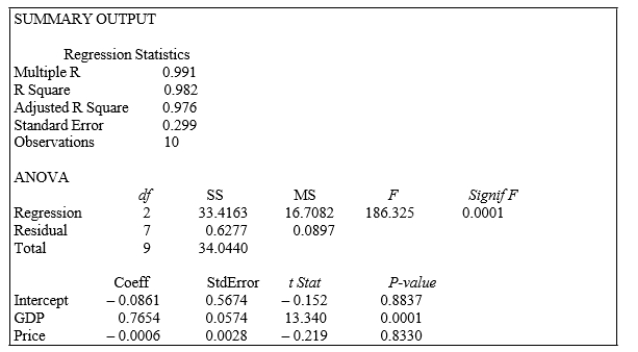-Referring to SCENARIO 13-3, the p-value for GDP is

(Multiple Choice)

4.7/5

(33)

Question 144

SCENARIO 13-15 The superintendent of a school district wanted to predict the percentage of students passing a sixth- grade proficiency test.She obtained the data on percentage of students passing the proficiency test (% Passing), mean teacher salary in thousands of dollars (Salaries), and instructional spending per pupil in thousands of dollars (Spending) of 47 schools in the state. Following is the multiple regression output with Y = % Passing as the dependent variable, X1 = Salaries and X 2 = Spending: Regression Statistics Multiple R 0.4276 R Square 0.1828 Adjusted R Square 0.1457 Standard Error 5.7351 Observations 47 ANOVA df SS MS F Significance F Regression 2 323.8284 161.9142 4.9227 0.0118 Residual 44 1447.2094 32.8911 Total 46 1771.0378 Coefficients Standard Error t Stat P-value Lower 95\% Upper 95\% Intercept -72.9916 45.9106 -1.5899 0.1190 -165.5184 19.5352 Salary 2.7939 0.8974 3.1133 0.0032 0.9853 4.6025 Spending 0.3742 0.9782 0.3825 0.7039 -1.5972 2.3455 -Referring to SCENARIO 13-15, what are the numerator and denominator degrees of freedom, respectively, for the test statistic to determine whether there is a significant relationship between percentage of students passing the proficiency test and the entire set of explanatory variables?

(Short Answer)

4.8/5

(38)

Question 145

From the coefficient of multiple determination, you cannot detect the strength of the relationship between Y and any individual independent variable.

(True/False)

4.8/5

(33)

Question 146

SCENARIO 13-6 One of the most common questions of prospective house buyers pertains to the cost of heating in dollars (Y).To provide its customers with information on that matter, a large real estate firm used the following 2 variables to predict heating costs: the daily minimum outside temperature in degrees of Fahrenheit ( X1 ) and the amount of insulation in inches ( X 2 ).Given below is EXCEL output of the regression model. Regression Statistics Multiple R 0.5270 R Square 0.2778 Adjusted R Square 0.1928 Standard Error 40.9107 Observations 20 ANOVA df SS MS F Significance F Regression 2 10943.0190 5471.5095 3.2691 0.0629 Residual 17 28452.6027 1673.6825 Total 19 39395.6218 13-22 Multiple Regression Coefficients Standard Error t Stat P-volue Lower 95\% Upper 95\% Intercept 448.2925 90.7853 4.9379 0.0001 256.7522 639.8328 Temperature -2.7621 1.2371 -2.2327 0.0393 -5.3721 -0.1520 Insulation -15.9408 10.0638 -1.5840 0.1316 -37.1736 5.2919 Also SSR \mid =8343.3572 and SSR \mid =4199.2672 -Referring to SCENARIO 13-6, the value of the partial F test statistic is forH0: Variable X1 does not significantly improve the model after variable X2 has been includedH1: Variable X1 significantly improves the model after variable X2 has been included

(Short Answer)

4.7/5

(40)

Question 147

SCENARIO 13-4 A real estate builder wishes to determine how house size (House) is influenced by family income (Income) and family size (Size).House size is measured in hundreds of square feet and income is measured in thousands of dollars.The builder randomly selected 50 families and ran the multiple regression.Partial Microsoft Excel output is provided below: Regression Statistics Multiple R 0.8479 R Square 0.7189 Adjusted R Square 0.7069 Standard Error 17.5571 Observations 50 $\text { ANOVA }$ df SS MS F Significance F Regression 37043.3236 18521.6618 0.0000 Residual 14487.7627 308.2503 Total 49 51531.0863 Coefficients Standard Error t Stat P-value Intercept -5.5146 7.2273 -0.7630 0.4493 Income 0.4262 0.0392 10.8668 0.0000 Size 5.5437 1.6949 3.2708 0.0020 $\text { Also } \operatorname{SSR}\left(X_{1} \mid X_{2}\right)=36400.6326 \text { and } \operatorname{SSR}\left(X_{2} \mid X_{1}\right)=3297.7917$ -Referring to SCENARIO 13-4, what annual income (in thousands of dollars) would an individual with a family size of 9 need to attain a predicted 5,000 square foot home (House = 50)?

(Short Answer)

4.7/5

(34)

Question 148

SCENARIO 13-3 An economist is interested to see how consumption for an economy (in $ billions) is influenced by gross domestic product ($ billions) and aggregate price (consumer price index).The Microsoft Excel output of this regression is partially reproduced below. -Referring to SCENARIO 13-3, when the economist used a simple linear regression model with consumption as the dependent variable and GDP as the independent variable, he obtained an r2 value of 0.971.What additional percentage of the total variation of consumption has been explained by including aggregate prices in the multiple regression?

(Multiple Choice)

4.7/5

(35)

Question 149

SCENARIO 13-7 The department head of the accounting department wanted to see if she could predict the GPA of students using the number of course units and total SAT scores of each.She takes a sample of 6 students and generates the following Microsoft Excel output: SUMMARY OUTPUT Regression Statistics Multiple R 0.916 R Square 0.839 Adjusted R Square 0.732 Standard Error 0.24685 Observations 6 ANOVA df SS MS F Signif F Regression 2 0.95219 0.47610 7.813 0.0646 Residual 3 0.18281 0.06094 Total 5 1.13500 Coeff StdError t Stat P -value Intercept 4.593897 1.13374542 4.052 0.0271 Units -0.247270 0.06268485 -3.945 0.0290 Total SAT 0.001443 0.00101241 1.425 0.2494 -Referring to SCENARIO 13-7, the department head wants to use a t test to test for the significance of the coefficient of X1.At a level of significance of 0.05, the departmenthead would decide that $\beta$ 1 $\neq$ 0 .

(True/False)

4.8/5

(30)

Question 150

A regression had the following results: SST = 82.55, SSE = 29.85.It can be said that 73.4% of the variation in the dependent variable is explained by the independent variables in the regression.

(True/False)

4.8/5

(33)

Question 151

SCENARIO 13-13 An econometrician is interested in evaluating the relationship of demand for building materials to mortgage rates in Los Angeles and San Francisco.He believes that the appropriate model is $Y = 10 + 5 X _ { 1 } + 8 X _ { 2 }$ where = mortgage rate in \% =1 if SF, 0 if LA Y= demand in \ 100 per capita -Referring to SCENARIO 13-13, the predicted demand in San Francisco when the mortgage rate is 10% is _.

(Short Answer)

4.8/5

(29)

Question 152

SCENARIO 13-4 A real estate builder wishes to determine how house size (House) is influenced by family income (Income) and family size (Size).House size is measured in hundreds of square feet and income is measured in thousands of dollars.The builder randomly selected 50 families and ran the multiple regression.Partial Microsoft Excel output is provided below: Regression Statistics Multiple R 0.8479 R Square 0.7189 Adjusted R Square 0.7069 Standard Error 17.5571 Observations 50 $\text { ANOVA }$ df SS MS F Significance F Regression 37043.3236 18521.6618 0.0000 Residual 14487.7627 308.2503 Total 49 51531.0863 Coefficients Standard Error t Stat P-value Intercept -5.5146 7.2273 -0.7630 0.4493 Income 0.4262 0.0392 10.8668 0.0000 Size 5.5437 1.6949 3.2708 0.0020 $\text { Also } \operatorname{SSR}\left(X_{1} \mid X_{2}\right)=36400.6326 \text { and } \operatorname{SSR}\left(X_{2} \mid X_{1}\right)=3297.7917$ -Referring to SCENARIO 13-4, _% of the variation in the house size can be explained by the variation in the family size while holding the family income constant.

(Short Answer)

4.9/5

(30)

Question 153

SCENARIO 13-15 The superintendent of a school district wanted to predict the percentage of students passing a sixth- grade proficiency test.She obtained the data on percentage of students passing the proficiency test (% Passing), mean teacher salary in thousands of dollars (Salaries), and instructional spending per pupil in thousands of dollars (Spending) of 47 schools in the state. Following is the multiple regression output with Y = % Passing as the dependent variable, X1 = Salaries and X 2 = Spending: Regression Statistics Multiple R 0.4276 R Square 0.1828 Adjusted R Square 0.1457 Standard Error 5.7351 Observations 47 ANOVA df SS MS F Significance F Regression 2 323.8284 161.9142 4.9227 0.0118 Residual 44 1447.2094 32.8911 Total 46 1771.0378 Coefficients Standard Error t Stat P-value Lower 95\% Upper 95\% Intercept -72.9916 45.9106 -1.5899 0.1190 -165.5184 19.5352 Salary 2.7939 0.8974 3.1133 0.0032 0.9853 4.6025 Spending 0.3742 0.9782 0.3825 0.7039 -1.5972 2.3455 -Referring to SCENARIO 13-15, what are the lower and upper limits of the 95% confidence interval estimate for the effect of a one thousand dollars increase in instructional spending per pupil on the mean percentage of students passing the proficiency test?

(Short Answer)

5.0/5

(31)

Question 154

SCENARIO 13-17 Given below are results from the regression analysis where the dependent variable is the number of weeks a worker is unemployed due to a layoff (Unemploy) and the independent variables are the age of the worker (Age) and a dummy variable for management position (Manager: 1 = yes, 0 = no). The results of the regression analysis are given below: Regression Statistics Multiple R 0.6391 R Square 0.4085 Adjusted R Square 0.3765 Standard Error 18.8929 Observations 40 ANOVA df SS MS F Significance F Regression 2 9119.0897 4559.5448 12.7740 0.0000 Residual 37 13206.8103 356.9408 Total 39 22325.9 Coefficients Standard Error t Stat P -value Intercept -0.2143 11.5796 -0.0185 0.9853 Age 1.4448 0.3160 4.5717 0.0000 Manager -22.5761 11.3488 -1.9893 0.0541 -Referring to SCENARIO 13-17, what are the lower and upper limits of the 95% confidence interval estimate for the difference in the mean number of weeks a worker is unemployed due to a layoff between a worker who is in a management position and one who is not after taking into consideration the effect of all the other independent variables?

(Short Answer)

4.9/5

(21)

Question 155

SCENARIO 13-15 The superintendent of a school district wanted to predict the percentage of students passing a sixth- grade proficiency test.She obtained the data on percentage of students passing the proficiency test (% Passing), mean teacher salary in thousands of dollars (Salaries), and instructional spending per pupil in thousands of dollars (Spending) of 47 schools in the state. Following is the multiple regression output with Y = % Passing as the dependent variable, X1 = Salaries and X 2 = Spending: Regression Statistics Multiple R 0.4276 R Square 0.1828 Adjusted R Square 0.1457 Standard Error 5.7351 Observations 47 ANOVA df SS MS F Significance F Regression 2 323.8284 161.9142 4.9227 0.0118 Residual 44 1447.2094 32.8911 Total 46 1771.0378 Coefficients Standard Error t Stat P-value Lower 95\% Upper 95\% Intercept -72.9916 45.9106 -1.5899 0.1190 -165.5184 19.5352 Salary 2.7939 0.8974 3.1133 0.0032 0.9853 4.6025 Spending 0.3742 0.9782 0.3825 0.7039 -1.5972 2.3455 -Referring to SCENARIO 13-15, there is sufficient evidence that the percentage of students passing the proficiency test depends on at least one of the explanatory variables at a5% level of significance.

(True/False)

4.7/5

(28)

Question 156

SCENARIO 13-15 The superintendent of a school district wanted to predict the percentage of students passing a sixth- grade proficiency test.She obtained the data on percentage of students passing the proficiency test (% Passing), mean teacher salary in thousands of dollars (Salaries), and instructional spending per pupil in thousands of dollars (Spending) of 47 schools in the state. Following is the multiple regression output with Y = % Passing as the dependent variable, X1 = Salaries and X 2 = Spending: Regression Statistics Multiple R 0.4276 R Square 0.1828 Adjusted R Square 0.1457 Standard Error 5.7351 Observations 47 ANOVA df SS MS F Significance F Regression 2 323.8284 161.9142 4.9227 0.0118 Residual 44 1447.2094 32.8911 Total 46 1771.0378 Coefficients Standard Error t Stat P-value Lower 95\% Upper 95\% Intercept -72.9916 45.9106 -1.5899 0.1190 -165.5184 19.5352 Salary 2.7939 0.8974 3.1133 0.0032 0.9853 4.6025 Spending 0.3742 0.9782 0.3825 0.7039 -1.5972 2.3455 -Referring to SCENARIO 13-15, which of the following is the correct alternative hypothesis to test whether instructional spending per pupil has any effect on percentage of students passing the proficiency test, considering the effect of mean teacher salary?

(Multiple Choice)

4.8/5

(36)

Question 157

SCENARIO 13-4 A real estate builder wishes to determine how house size (House) is influenced by family income (Income) and family size (Size).House size is measured in hundreds of square feet and income is measured in thousands of dollars.The builder randomly selected 50 families and ran the multiple regression.Partial Microsoft Excel output is provided below: Regression Statistics Multiple R 0.8479 R Square 0.7189 Adjusted R Square 0.7069 Standard Error 17.5571 Observations 50 $\text { ANOVA }$ df SS MS F Significance F Regression 37043.3236 18521.6618 0.0000 Residual 14487.7627 308.2503 Total 49 51531.0863 Coefficients Standard Error t Stat P-value Intercept -5.5146 7.2273 -0.7630 0.4493 Income 0.4262 0.0392 10.8668 0.0000 Size 5.5437 1.6949 3.2708 0.0020 $\text { Also } \operatorname{SSR}\left(X_{1} \mid X_{2}\right)=36400.6326 \text { and } \operatorname{SSR}\left(X_{2} \mid X_{1}\right)=3297.7917$ -Referring to SCENARIO 13-4, which of the following values for the level of significance is the smallest for which at most one explanatory variable is significant individually?

(Multiple Choice)

4.9/5

(43)

Question 158

SCENARIO 13-17 Given below are results from the regression analysis where the dependent variable is the number of weeks a worker is unemployed due to a layoff (Unemploy) and the independent variables are the age of the worker (Age) and a dummy variable for management position (Manager: 1 = yes, 0 = no). The results of the regression analysis are given below: Regression Statistics Multiple R 0.6391 R Square 0.4085 Adjusted R Square 0.3765 Standard Error 18.8929 Observations 40 ANOVA df SS MS F Significance F Regression 2 9119.0897 4559.5448 12.7740 0.0000 Residual 37 13206.8103 356.9408 Total 39 22325.9 Coefficients Standard Error t Stat P -value Intercept -0.2143 11.5796 -0.0185 0.9853 Age 1.4448 0.3160 4.5717 0.0000 Manager -22.5761 11.3488 -1.9893 0.0541 -Referring to SCENARIO 13-17, there is sufficient evidence that at least one of the explanatory variables is related to the number of weeks a worker is unemployed due to a layoff at a 10% level of significance.

(True/False)

4.9/5

(38)

Question 159

Only when all three of the hat matrix elements hi, the Studentized deleted residuals ti and the Cook's distance statistic Di reveal consistent result should an observation be removed from the regression analysis.

(True/False)

4.8/5

(43)

Question 160

In a multiple regression model, which of the following is correct regarding the value of the adjusted r 2 ?

From the coefficient of multiple determination, you cannot detect the strength of the relationship between Y and any individual independent variable.

A regression had the following results: SST = 82.55, SSE = 29.85.It can be said that 73.4% of the variation in the dependent variable is explained by the independent variables in the regression.

Only when all three of the hat matrix elements hi, the Studentized deleted residuals ti and the Cook's distance statistic Di reveal consistent result should an observation be removed from the regression analysis.

Defining and Collecting Data

Organizing and Visualizing Variables

Numerical Descriptive Measures

Basic Probability

Discrete Probability Distributions

The Normal Distribution

Sampling Distributions

Confidence Interval Estimation

Fundamentals of Hypothesis Testing: One-Sample Tests

Two-Sample Tests

Chi-Square Tests

Simple Linear Regression

Business Analytics

Filters