Exam 5: Regression With a Single Regressor: Hypothesis Tests and Confidence Intervals

Under the least squares assumptions (zero conditional mean for the error term, Xi and Yi being i.i.d., and Xi and ui having finite fourth moments), the OLS estimator For the slope and intercept a. has an exact normal distribution for $n > 15$ . b. is BLUE. c. has a normal distribution even in small samples. d. is unbiased.

In many of the cases discussed in your textbook, you test for the significance of the slope at the 5% level.What is the size of the test? What is the power of the test? Why is the probability of committing a Type II error so large here?

Consider the following two models involving binary variables as explanatory variables: $\widehat { \text { Wage } } = \widehat { \beta } _ { 0 } + \widehat { \beta } _ { 1 } D \text { Femme and } \widehat { \text { Wage } } = \widehat { \phi } _ { 1 } D \text { Femme } + \widehat { \phi } _ { 2 } \text { Male }$ where Wage is the hourly wage rate, DFemme is a binary variable that is equal to 1 if the person is a female, and 0 if the person is a male. Male $= 1 -$ DFemme. Even though you have not learned about regression functions with two explanatory variables (or regressions without an intercept), assume that you had estimated both models, i.e., you obtained the estimates for the regression coefficients. What is the predicted wage for a male in the two models? What is the predicted wage for a female in the two models? What is the relationship between the $\beta \mathrm { s }$ and the $\phi s$ ? Why would you prefer one model over the other?

For the following estimated slope coefficients and their heteroskedasticity robust standard errors, find the t -statistics for the null hypothesis $H _ { 0 } : \beta _ { 1 } = 0$ Assuming that your sample has more than 100 observations, indicate whether or not you are able to reject the null hypothesis at the 10 %, 5 % , and 1 % level of a one-sided and two-sided hypothesis. (a) $\hat { \beta } _ { 1 } = 4.2 , S E \left( \hat { \beta } _ { 1 } \right) = 2.4$ (b) $\hat { \beta } _ { 1 } = 0.5 , S E \left( \hat { \beta } _ { 1 } \right) = 0.37$ (c) $\hat { \beta } _ { 1 } = 0.003 , S E \left( \hat { \beta } _ { 1 } \right) = 0.002$ (d) $\hat { \beta } _ { 1 } = 360 , S E \left( \hat { \beta } _ { 1 } \right) = 300$

If the absolute value of your calculated t-statistic exceeds the critical value from the standard normal distribution, you can

(continuation with the Purchasing Power Parity question from Chapter 4) The news-magazine The Economist regularly publishes data on the so called Big Mac index and exchange rates between countries.The data for 30 countries from the April 29, 2000 issue is listed below: 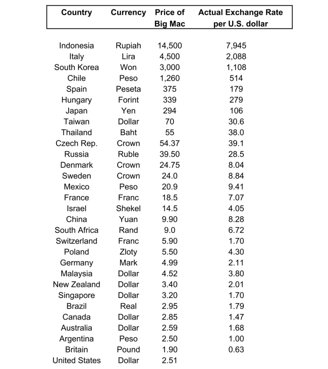The concept of purchasing power parity or PPP ("the idea that similar foreign and domestic goods ... should have the same price in terms of the same currency," Abel, A. and B. Bernanke, Macroeconomics, $4 ^ { \text {th } }$ edition, Boston: Addison Wesley, 476) suggests that the ratio of the Big Mac priced in the local currency to the U.S. dollar price should equal the exchange rate between the two countries. 16 After entering the data into your spread sheet program, you calculate the predicted exchange rate per U.S.dollar by dividing the price of a Big Mac in local currency by the U.S.price of a Big Mac ($2.51).To test for PPP, you regress the actual exchange rate on the predicted exchange rate. The estimated regression is as follows: -27.05+1.35\times Pr edExRate =0.994,n=29,SER=122.15 (23.74) (0.02) (a)Your spreadsheet program does not allow you to calculate heteroskedasticity robust standard errors.Instead, the numbers in parenthesis are homoskedasticity only standard errors.State the two null hypothesis under which PPP holds.Should you use a one-tailed or two-tailed alternative hypothesis?

You recall from one of your earlier lectures in macroeconomics that the per capita income depends on the savings rate of the country: those who save more end up with a higher standard of living.To test this theory, you collect data from the Penn World Tables on GDP per worker relative to the United States (RelProd)in 1990 and the average investment share of GDP from 1980-1990 (sK ), remembering that investment equals saving.The regression results in the following output: =0.08+2.44\times,=0.46,SER=0.21 (0.04)(0.38) (a)Interpret the regression results carefully.

The effect of decreasing the student-teacher ratio by one is estimated to result in an improvement of the districtwide score by 2.28 with a standard error of 0.52. Construct a 90% and 99% confidence interval for the size of the slope coefficient and the corresponding predicted effect of changing the student-teacher ratio by one.What is the intuition on why the 99% confidence interval is wider than the 90% confidence interval?

Assume that the homoskedastic normal regression assumption hold.Using the Student t-distribution, find the critical value for the following situation: (a) $\quad n = 28,5 \%$ significance level, one-sided test. (b) $\quad n = 40,1 \%$ significance level, two-sided test. (c) $n = 10,10 \%$ significance level, one-sided test. (d) $n = \infty , 5 \%$ significance level, two-sided test.

In order to formulate whether or not the alternative hypothesis is one-sided or two-sided, you need some guidance from economic theory.Choose at least three examples from economics or other fields where you have a clear idea what the null hypothesis and the alternative hypothesis for the slope coefficient should be. Write a brief justification for your answer.

Changing the units of measurement obviously will have an effect on the slope of your regression function. For example, let $Y ^ { * } = a Y \text { and } X ^ { * } = b X \text {. }$ Then it is easy but tedious to show that $\widehat { \beta } _ { 1 } ^ { * } = \frac { \sum _ { i = 1 } ^ { n } x _ { i } ^ { * } y _ { i } ^ { * } } { \sum _ { i = 1 } ^ { n } x _ { i } ^ { * 2 } } = \frac { a } { b } \widehat { \beta } _ { 1 }$ Given this result, how do you think the standard errors and the regression $R ^ { 2 }$ will change?

Your textbook discussed the regression model when X is a binary variable $Y _ { i } = \beta _ { 0 } + \beta _ { 1 } D _ { i } + u _ { i } , i = 1 , \ldots , n$ Let $Y$ represent wages, and let $D$ be one for females, and 0 for males. Using the OLS formula for the intercept coefficient, prove that $\widehat { \beta } _ { 0 }$ is the average wage for males.

(Continuation from Chapter 4, number 6)The neoclassical growth model predicts that for identical savings rates and population growth rates, countries should converge to the per capita income level.This is referred to as the convergence hypothesis.One way to test for the presence of convergence is to compare the growth rates over time to the initial starting level. (a)The results of the regression for 104 countries were as follows: = 0.019-0.0006\times,=0.00007,SER=0.016 (0.004)(0.0073) where $g 6090$ is the average annual growth rate of GDP per worker for the $1960 -$ 1990 sample period, and $\operatorname { RelProd } _ { 60 }$ is GDP per worker relative to the United States in 1960. Numbers in parenthesis are heteroskedasticity robust standard errors. Using the OLS estimator with homoskedasticity-only standard errors, the results changed as follows: = 0.019-0.0006\times,=0.00007,SER=0.016 (0.002)(0.0068) Why didn't the estimated coefficients change? Given that the standard error of the slope is now smaller, can you reject the null hypothesis of no beta convergence? Are the results in the second equation more reliable than the results in the first equation? Explain.