Exam 5: Regression With a Single Regressor: Hypothesis Tests and Confidence Intervals

You have obtained measurements of height in inches of 29 female and 81 male students (Studenth)at your university.A regression of the height on a constant and a binary variable (BFemme), which takes a value of one for females and is zero otherwise, yields the following result: = 71.0-4.84\times BFemme ,=0.40,SER=2.0 (0.3)(0.57) (a)What is the interpretation of the intercept? What is the interpretation of the slope? How tall are females, on average?

Consider the sample regression function $\widehat { Y } _ { i } = \widehat { \beta } _ { 0 } + \widehat { \beta } _ { 1 } X _ { i }$ The table below lists estimates for the slope $\left( \widehat { \beta } _ { 1 } \right)$ and the variance of the slope estimator $\left( \widehat { \sigma } _ { \widehat { \beta } _ { 1 } } ^ { 2 } \right)$ In each case calculate the p -value for the null hypothesis of $\beta _ { 1 } = 0$ and a two-tailed alternative hypothesis. Indicate in which case you would reject the null hypothesis at the 5 % significance level. -1.76 0.0025 2.85 -0.00014 0.37 0.000003 117.5 0.0000013

Imagine that you were told that the t -statistic for the slope coefficient of the regression line $\widehat { \text { TestScore } } = 698.9 - 2.28 \times S T R$ was 4.38 . What are the units of measurement for the t -statistic?

Assume that your population regression function is $Y _ { i } = \beta _ { 1 } X _ { i } + u _ { i }$ i.e., a regression through the origin (no intercept).Under the homoskedastic normal regression assumptions, the t-statistic will have a Student t distribution with n-1 degrees of freedom, not n-2 degrees of freedom, as was the case in Chapter 5 of your textbook.Explain.Do you think that the residuals will still sum to zero for this case?

(continuation from Chapter 4) Sir Francis Galton, a cousin of James Darwin, examined the relationship between the height of children and their parents towards the end of the $19 ^ { \text {th } }$ century. It is from this study that the name "regression" originated. You decide to update his findings by collecting data from 110 college students, and estimate the following relationship: = 19.6+0.73\times Midparh, =0.45,SER=2.0 (7.2)(0.10) where Studenth is the height of students in inches, and Midparh is the average of the parental heights.Values in parentheses are heteroskedasticity robust standard errors.(Following Galton's methodology, both variables were adjusted so that the average female height was equal to the average male height.) (a)Test for the statistical significance of the slope coefficient.

(Requires Appedix material and Calculus) Equation (5.36) in your textbook derives the conditional variance for any old conditionally unbiased estimator $\widetilde { \beta } _ { 1 }$ to be $\operatorname { var } \left( \widetilde { \beta } _ { 1 } \mid X _ { 1 } , \ldots , X _ { n } \right) = \sigma _ { u } ^ { 2 } \sum _ { i = 1 } ^ { n } a _ { i } ^ { 2 }$ (where the conditions for conditional unbiasedness are $\sum _ { i = 1 } ^ { n } a _ { i } = 0$ and $\sum _ { i = 1 } ^ { n } a _ { i } X _ { i } = 1$ . As an alternative to the BLUE proof presented in your textbook, you recall from one of your calculus courses that you could minimize the variance subject to the two constraints, thereby making the variance as small as possible while the constraints are holding. Show that in doing so you get the OLS weights $\hat { a } _ { i }$ . (You may assume that $X _ { 1 } , \ldots , X _ { n }$ are nonrandom (fixed over repeated samples.)) 22

The neoclassical growth model predicts that for identical savings rates and population growth rates, countries should converge to the per capita income level. This is referred to as the convergence hypothesis. One way to test for the presence of convergence is to compare the growth rates over time to the initial starting level, i.e., to run the regression $\widehat { g 6090 } = \widehat { \beta _ { 0 } } + \widehat { \beta _ { 1 } } \times \operatorname { RelProd } _ { 60 }$ , where $g 6090$ is the average annual growth rate of GDP per worker for the 1960-1990 sample period, and $\operatorname { RelProd } _ { 60 }$ is GDP per worker relative to the United States in 1960. Under the null hypothesis of no convergence, $\beta _ { 1 } = 0 ; H _ { 1 } : \beta _ { 1 } < 0$ , implying ("beta") convergence. Using a standard regression package, you get the following output: Dependent Variable: G6090 Method: Least Squares Date: 07/11/06 Time: 05:46 Sample: 1104 Included observations: 104 White Heteroskedasticity-Consistent Standard Errors & Covariance 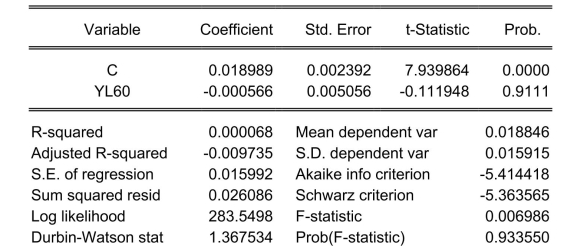You are delighted to see that this program has already calculated p-values for you. However, a peer of yours points out that the correct p-value should be 0.4562. Who is right?

The only difference between a one- and two-sided hypothesis test is

Your textbook discussed the regression model when X is a binary variable $Y _ { i } = \beta _ { 0 } + \beta _ { 1 } D _ { i } + u _ { i } , i = 1 , \ldots , n$ Let $Y$ represent wages, and let $D$ be one for females, and 0 for males. Using the OLS formula for the slope coefficient, prove that $\widehat { \beta } _ { 1 }$ is the difference between the average wage for males and the average wage for females.

(continuation from Chapter 4, number 3)You have obtained a sub-sample of 1744 individuals from the Current Population Survey (CPS)and are interested in the relationship between weekly earnings and age.The regression, using heteroskedasticity-robust standard errors, yielded the following result: = 239.16+5.20\times Age ,=0.05, SER =287.21., (20.24)(0.57) where Earn and Age are measured in dollars and years respectively. (a)Is the relationship between Age and Earn statistically significant?

The proof that OLS is BLUE requires all of the following assumptions with the exception of: a. the errors are homoskedastic. b. the errors are normally distributed. c. $E \left( u _ { i } \mid X _ { i } \right) = 0$ . d. large outliers are unlikely.

In general, the t-statistic has the following form: a. $\frac { \text { estimate-hypothesize value } } { \text { standard error of estimate } }$ . b. $\frac { \text { estimator } } { \text { standard error of estimator } }$ . c. $\frac { \text { estimator-hypothesize value } } { \text { standard error of estimator } }$ . d. $\frac{\frac{\text { estimator-hypothesize value }}{\text { standard error of estimator }}}{\sqrt{\mathrm{n}}} \text {. }$

Consider the following regression line: $\widehat { \text { TestScore } } = 698.9 - 2.28 \times \text { STR }$ You are told that the t -statistic on the slope coefficient is 4.38 . What is the standard error of the slope coefficient?

The 95% confidence interval for $\beta _ { 1 }$ is the interval

The homoskedasticity-only estimator of the variamce of $\widehat { \beta } _ { 1 }$ is

The t-statistic is calculated by dividing

With heteroskedastic errors, the weighted least squares estimator is BLUE.You should use OLS with heteroskedasticity-robust standard errors because

Carefully discuss the advantages of using heteroskedasticity-robust standard errors over standard errors calculated under the assumption of homoskedasticity. Give at least five examples where it is very plausible to assume that the errors display heteroskedasticity.

One of the following steps is not required as a step to test for the null hypothesis: a. compute the standard error of $\widehat { \beta } _ { 1 }$ . b. test for the errors to be normally distributed. c. compute the $t$ -statistic. d. compute the $p$ -value.

Finding a small value of the p-value (e.g.less than 5%)