Exam 4: Linear Regression With One Regressor

(Requires Appendix material)Consider the sample regression function $Y _ { i } ^ { * } = \hat { \gamma } _ { 0 } + \hat { \gamma } _ { 1 } X _ { i } ^ { * } + \hat { u } _ { i }$ where "*" indicates that the variable has been standardized. What are the units of measurement for the dependent and explanatory variable? Why would you want to transform both variables in this way? Show that the OLS estimator for the intercept equals zero. Next prove that the OLS estimator for the slope in this case is identical to the formula for the least squares estimator where the variables have not been standardized, times the ratio of the sample standard deviation of $X$ and $Y$ , i.e., $\hat { \gamma } _ { 1 } = \hat { \beta } _ { 1 } * \frac { s _ { X } } { s _ { Y } }$ .

The help function for a commonly used spreadsheet program gives the following definition for the regression slope it estimates: $\frac { n \sum _ { i = 1 } ^ { n } X _ { i } Y _ { i } - \left( \sum _ { i = 1 } ^ { n } X _ { i } \right) \left( \sum _ { i = 1 } ^ { n } Y _ { i } \right) } { n \sum _ { i = 1 } ^ { n } X _ { i } ^ { 2 } - \left( \sum _ { i = 1 } ^ { n } X _ { i } \right) ^ { 2 } }$ Prove that this formula is the same as the one given in the textbook.

The baseball team nearest to your home town is, once again, not doing well.Given that your knowledge of what it takes to win in baseball is vastly superior to that of management, you want to find out what it takes to win in Major League Baseball (MLB). You therefore collect the winning percentage of all 30 baseball teams in MLB for 1999 and regress the winning percentage on what you consider the primary determinant for wins, which is quality pitching (team earned run average).You find the following information on team performance: 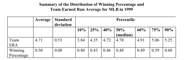(a)What is your expected sign for the regression slope? Will it make sense to interpret the intercept? If not, should you omit it from your regression and force the regression line through the origin?

The regression $R ^ { 2 }$ is defined as follows:

Indicate in a scatterplot what the data for your dependent variable and your explanatory variable would look like in a regression with an R² equal to zero. How would this change if the regression R² was equal to one?

You have analyzed the relationship between the weight and height of individuals. Although you are quite confident about the accuracy of your measurements, you feel that some of the observations are extreme, say, two standard deviations above and below the mean.Your therefore decide to disregard these individuals.What consequence will this have on the standard deviation of the OLS estimator of the slope?

Binary variables

Prove that the regression $R ^ { 2 }$ is identical to the square of the correlation coefficient between two variables Y and X . Regression functions are written in a form that suggests causation running from X to Y . Given your proof, does a high regression $R ^ { 2 }$ present supportive evidence of a causal relationship? Can you think of some regression examples where the direction of causality is not clear? Is without a doubt?

The slope estimator, $\beta _ { 1 }$ has a smaller standard error, other things equal, if

(Requires Appendix material)At a recent county fair, you observed that at one stand people's weight was forecasted, and were surprised by the accuracy (within a range). Thinking about how the person could have predicted your weight fairly accurately (despite the fact that she did not know about your "heavy bones"), you think about how this could have been accomplished.You remember that medical charts for children contain 5%, 25%, 50%, 75% and 95% lines for a weight/height relationship and decide to conduct an experiment with 110 of your peers.You collect the data and calculate the following sums: =17,375,=7,665.5 =94,228.8,=1,248.9,=7,625.9 where the height is measured in inches and weight in pounds. (Small letters refer to deviations from means as in $z _ { i } = Z _ { i } - \bar { Z }$ .) (a)Calculate the slope and intercept of the regression and interpret these.

To decide whether or not the slope coefficient is large or small,

In order to calculate the slope, the intercept, and the regression $R ^ { 2 }$ for a simple sample regression function, list the five sums of data that you need.

(Requires Appendix material) In deriving the OLS estimator, you minimize the sum of squared residuals with respect to the two parameters $\hat { \beta } _ { 0 } \text { and } \hat { \beta } _ { 1 }$ . The resulting two equations imply two restrictions that OLS places on the data, namely that $\sum _ { i = 1 } ^ { n } \hat { u } _ { i } = 0$ and $\sum _ { i = 1 } ^ { n } \hat { u } _ { i } X _ { i } = 0$ Show that you get the same formula for the regression slope and the intercept if you impose these two conditions on the sample regression function.

Interpreting the intercept in a sample regression function is

In the linear regression model, $Y _ { i } = \beta _ { 0 } + \beta _ { 1 } X _ { i } + u _ { i } , \beta _ { 0 } + \beta _ { 1 } X _ { i }$ is referred to as

The OLS slope estimator is not defined if there is no variation in the data for the explanatory variable.You are interested in estimating a regression relating earnings to years of schooling.Imagine that you had collected data on earnings for different individuals, but that all these individuals had completed a college education (16 years of education).Sketch what the data would look like and explain intuitively why the OLS coefficient does not exist in this situation.

The OLS estimator is derived by

(Requires Appendix material) A necessary and sufficient condition to derive the OLS estimator is that the following two conditions hold: $\sum _ { i = 1 } ^ { n } \hat { u } _ { i } = 0 \text { and } \sum _ { i = 1 } ^ { n } \hat { u } _ { i } X _ { i } = 0$ Show that these conditions imply that $\sum _ { i = 1 } ^ { n } \hat { u } _ { i } \hat { Y } _ { i } = 0$

For the simple regression model of Chapter 4, you have been given the following data: =274,745.75;=8,248.979; =5,392,705;=163,513.03;=179,878,841.13 (a)Calculate the regression slope and the intercept.

(Requires Calculus)Consider the following model: $Y _ { i } = \beta _ { 0 } + u _ { i } .$ Derive the OLS estimator for $\beta _ { 0 }$ .