Exam 14: Introduction to Time Series Regression and Forecasting

The Granger Causality Test c. uses the $F$ -statistic to test the hypothesis that certain regressors have no predictive content for the dependent variable beyond that contained in the other regressors. d. establishes the direction of causality (as used in common parlance) between $X$ and $Y$ in addition to correlation. e. is a rather complicated test for statistical independence. f. is a special case of the Augmented Dickey-Fuller test.

You should use the QLR test for breaks in the regression coefficients, when

Time series variables fail to be stationary when

Autoregressive distributed lag models include

Stationarity means that the

The Times Series Regression with Multiple Predictors a. is the same as the $\operatorname { ADL } ( p , q )$ with additional predictors and their lags present. b. gives you more than one prediction. c. cannot be estimated by OLS due to the presence of multiple lags. d. requires that the $k$ regressors and the dependent variable have nonzero, finite eighth moments.

You want to determine whether or not the unemployment rate for the United States has a stochastic trend using the Augmented Dickey Fuller Test (ADF).The BIC suggests using 3 lags, while the AIC suggests 4 lags. (a)Which of the two will you use for your choice of the optimal lag length?

One of the sources of error in the RMSFE in the AR(1) model is

Having learned in macroeconomics that consumption depends on disposable income, you want to determine whether or not disposable income helps predict future consumption. You collect data for the sample period 1962:I to 1995:IV and plot the two variables. (a)To determine whether or not past values of personal disposable income growth rates help to predict consumption growth rates, you estimate the following relationship. 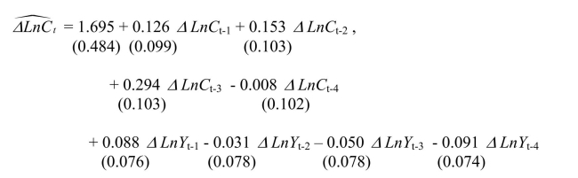The Granger causality test for the exclusion on all four lags of the GDP growth rate is 0.98.Find the critical value for the 1%, the 5%, and the 10% level from the relevant table and make a decision on whether or not these additional variables Granger cause the change in the growth rate of consumption.

If a "break" occurs in the population regression function, then

In order to make reliable forecasts with time series data, all of the following conditions are needed with the exception of

One reason for computing the logarithms (ln), or changes in logarithms, of economic time series is that

$\text { Consider the AR(1) model } Y _ { t } = \beta _ { 0 } + \beta _ { 1 } Y _ { t - 1 } + u _ { t } , \left| \beta _ { 1 } \right| < 1 \text {.. }$ (a) $\text { Find the mean and variance of } Y _ { t } \text {. }$

The root mean squared forecast error (RMSFE)is defined as a. $\sqrt { E \left[ \left| Y _ { T } - \hat { Y } _ { T \mid T - 1 } \right| \right] }$ . b. $\sqrt { E \left[ \left( Y _ { T + 1 } - \hat { Y } _ { T + 1 T } \right) ^ { 2 } \right] }$ . c. $\sqrt { \left( Y _ { T } - \hat { Y } _ { T \mid T - 1 } \right) ^ { 2 } }$ . d. $\sqrt { E \left[ \left( Y _ { T } - \hat { Y } _ { T \mid T - 1 } \right) \right] }$ .

Negative autocorrelation in the change of a variable implies that

The forecast is