Exam 12: Multiple Regression and Model Building
Exam 1: Statistics, Data, and Statistical Thinking74 Questions
Exam 2: Methods for Describing Sets of Data188 Questions
Exam 3: Probability237 Questions
Exam 4: Random Variables and Probability Distributions273 Questions
Exam 5: Sampling Distributions52 Questions
Exam 6: Inferences Based on a Single Sample: Estimation With Confidence Intervals135 Questions
Exam 7: Inferences Based on a Single Sample: 355 Tests of Hypotheses144 Questions
Exam 8: Inferences Based on Two Samples: Confidence Intervals and Tests of Hypotheses102 Questions
Exam 9: Design of Experiments and Analysis of Variance87 Questions
Exam 10: Categorical Data Analysis59 Questions
Exam 11: Simple Linear Regression113 Questions
Exam 12: Multiple Regression and Model Building131 Questions
Exam 13: Methods for Quality Improvement: Statistical Process Control Available on CD89 Questions
Exam 14: Time Series: Descriptive Analyses, Models, and Forecasting Available on CD73 Questions
Exam 15: Nonparametric Statistics Available on CD49 Questions
Select questions type
What relationship between x and y is suggested by the scattergram? 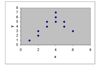
Free
(Multiple Choice)
4.8/5  (36)
(36)
Correct Answer: Verified
A
An elections officer wants to model voter turnout (y) in a precinct as a function of type of election, national or state.
Write a model for mean voter turnout, E(y), as a function of type of election.
Free
(Multiple Choice)
4.8/5 (45)
Correct Answer:Verified
A
Consider the model where is a quantitative variable and and are dummy variables describing a qualitative variable at three levels using the coding scheme
The resulting least squares prediction equation is . What is the least squares regression equation associated with level 2?
Free
(Multiple Choice)
4.9/5 (39)
Correct Answer:Verified
D
The sum of squared errors (SSE) of a least squares regression model decreases when new terms are added to the model.
(True/False)
4.7/5 (45)
In stepwise regression, the probability of making one or more Type I or Type II errors is quite small.
(True/False)
4.9/5 (40)
A study of the top MBA programs attempted to predict the average starting salary (in $1000's) of graduates of the program based on the amount of tuition (in $1000's) charged by the program and the average GMAT score of the program's students. The results of a regression analysis based on a sample of 75 MBA programs is shown below:
Least Squares Linear Regression of Salary
Predictor Variables Coefficient Std Error T P VIF Constant -203.402 51.6573 -3.94 0.0002 0.0 Gmat 0.39412 0.09039 4.36 0.0000 2.0 Tuition 0.92012 0.17875 5.15 0.0000 2.0
R-Squared 0.6857 Resid. Mean Square (MSE) 427.511 Adjusted R-Squared 0.6769 Standard Deviation 20.6763
Source DF SS MS F P Regression 2 67140.9 33570.5 78.53 0.0000 Residual 72 30780.8 427.5 Total 74 97921.7
(Multiple Choice)
4.9/5 (41)
The printout below shows part of the least squares regression analysis for the model fit to a set of data. The model attempts to predict a score on the final exam in a statistics course based on the scores on the first two tests in the class.
ANOVA
df SS MS F Significance F Regression 2 1293.125328 646.5626641 21.27366772 2.35769-05 Residual 17 516.6746719 30.39262776 Total 19 1809.8
Coefficients Standard Error t Stat P-value Lower 95\% Upper 95\% Intercept -4.409686163 16.72267106 -0.263695085 0.795184685 -39.69148734 30.87211502 Test 1 0.397435806 0.343012569 1.158662514 0.262611745 -0.326258467 1.121130079 Test 2 0.638805278 0.224623383 2.843894834 0.011217936 0.164890704 1.112719852
Is there evidence of multicollinearity in the printout? Explain.
(Essay)
4.8/5 (36)
For a multiple regression model, we assume that the mean of the probability distribution of the
random error is 0.
(True/False)
4.7/5 (37)
The model was fit to a set of data, and the following plot of residuals against values was obtained.
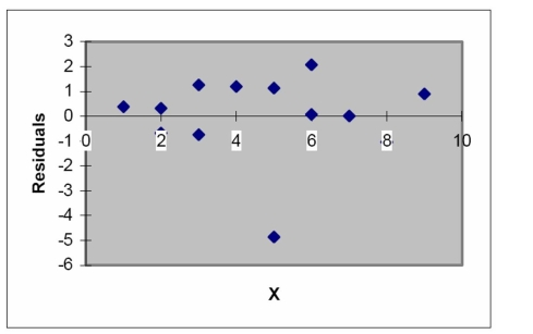 Interpret the residual plot.
(Essay)
4.9/5 (42)
A study of the top MBA programs attempted to predict the average starting salary (in $1000's) of graduates of the program based on the amount of tuition (in $1000's) charged by the program and the average GMAT score of the program's students. The results of a regression analysis based on a sample of 75 MBA programs is shown below: Least Squares Linear Regression of Salary Predictor Variables Coefficient Std Error T P Constant -687.851 165.406 4.16 0.0001 Tuition -11.3197 2.19724 -5.15 0.0000 GMAT -0.96727 0.25535 -3.79 0.0003
TxG 0.01850 0.00331 5.58 0.0000
R-Squared 0.7816 Resid. Mean Square (MSE) 301.251 Adjusted R-Squared 0.7723 Standard Deviation 17.3566
Source DF SS MS F P Regression 3 76523.8 25510.9 84.68 0.0000 Residual 71 21388.8 301.3 Total 74 97921.7
Cases Included 75 Missing Cases 0
The global-f test statistic is shown on the printout to be the value . Interpret this value.
(Multiple Choice)
4.8/5 (36)
The concessions manager at a beachside park recorded the high temperature, the number of people at the park, and the number of bottles of water sold for each of 12 consecutiveSaturdays. The data are shown below.
Bottles Sold Temperature People 341 73 1625 425 79 2100 457 80 2125 485 80 2800 469 81 2550 395 82 1975 511 83 2675 549 83 2800 543 85 2850 537 88 2775 621 89 2800 897 91 3100
a. Fit the model to the data, letting represent the number of bottles of water sold, the temperature, and the number of people at the park.
b. Identify at least two indicators of multicollinearity in the model.
c. Comment on the usefulness of the model to predict the number of bottles of water sold on a Saturday when the high temperature is and there are 3500 people at the park.
(Essay)
4.7/5 (35)
It is desired to build a regression model to predict the sales price of a single family home, based on the size of the house and the neighborhood the home is located in. The goal is to compare the prices of homes that are located in two different neighborhoods. The following model is proposed:
A regression model was fit and the following residual plot was observed.
Residual
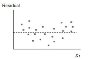 Which of the following assumptions appears violated based on this plot?
(Multiple Choice)
4.8/5 (36)
Consider the partial printout for an interaction regression analysis of the relationship between a dependent variable and two independent variables and .
ANOVA
df SS MS F Significance F Regression 3 3393.677324 1131.225775 9391.974782 2.11084-11 Residual 6 0.722675987 0.120445998 Total 9 3394.4
Coefficients Standard Error t Stat P-value Lower 95\% Upper 95\% Intercept 16.72197014 8.283997219 2.018587126 0.09007654 -3.548255659 36.99219593 -3.037317759 2.678748705 -1.133856921 0.300116382 -9.591984506 3.517348987 -1.046522754 1.547132645 -0.676427297 0.523973988 -4.832222727 2.73917722 4.071685147 0.444059933 9.169224345 9.47663-05 2.98510884 5.158261454
a. Write the prediction equation for the interaction model.
b. Test the overall utility of the interaction model using the global -test at .
c. Test the hypothesis (at ) that and interact positively.
d. Estimate the change in for each additional 1-unit increase in when .
(Essay)
4.8/5 (29)
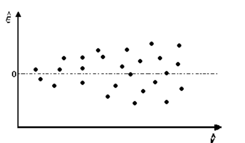
Suppose that the following model was fit to a set of data.
The corresponding plot if residuals against predicted values is shown. Interpret the plot.
(Multiple Choice)
4.8/5 (46)
Retail price data for hard disk drives were recently reported in a computer magazine. Three variables were recorded for each hard disk drive:
Retail PRICE (measured in dollars)
Microprocessor SPEED (measured in megahertz)
(Values in sample range from 10 to 40 )
size (measured in computer processing units)
(Values in sample range from 286 to 486 )
A first-order regression model was fit to the data. Part of the printout follows:
Dep Var Predict Std Err Lower 95\% Upper 95\% OBS SPEED CHIP PRICE Value Predict Predict Predict Residual 1 33 386 5099.0 4464.9 260.768 3942.7 4987.1 634.1
Interpret the prediction interval for when and .
(Essay)
4.9/5 (39)
Consider the second-order model
If is held fixed at , describe the relationship between and .
(Multiple Choice)
5.0/5 (44)
During its manufacture, a product is subjected to four different tests in sequential order. An efficiency expert claims that the fourth (and last) test is unnecessary since its results can be predicted based on the first three tests. To test this claim, multiple regression will be used to model Test4 score , as a function of Test1 score ), Test 2 score , and Test3 score . [Note: All test scores range from 200 to 800 , with higher scores indicative of a higher quality product.] Consider the model:
The first-order model was fit to the data for each of 12 units sampled from the production line. The results are summarized in the printout.
SOURCE DF SS MS FVALUE PROB > F MODEL 3 151417 50472 18.16 .0075 ERROR 8 22231 2779 TOTAL 12 173648
ROOT MSE 52.72 R-SQUARE 0.872 DEP MEAN 645.8 ADJ R-SQ 0.824
PARAMETER STANDARD T FOR 0: VARIABLES ESTIMATE ERROR PARAMETER =0 PROB >|T|
INTERCEPT 11.98 80.50 0.15 0.885 X1(TEST1) 0.2745 0.1111 2.47 0.039 X2(TEST2) 0.3762 0.0986 3.82 0.005 X3(TEST3) 0.3265 0.0808 4.04 0.004
Compute a confidence interval for .
(Multiple Choice)
4.7/5 (36)
The rejection of the null hypothesis in a global F-test means that the model is the best model for providing reliable estimates and predictions.
(True/False)
5.0/5 (38)
A collector of grandfather clocks believes that the price received for the clocks at an auction increases with the number of bidders, but at an increasing (rather than a constant) rate. Thus, the model proposed to best explain auction price (y, in dollars) by number of bidders (x) is the quadratic model
This model was fit to data collected for a sample of 32 clocks sold at auction.
Suppose the -value for the test of vs. is . What is the proper conclusion?
(Multiple Choice)
4.8/5 (39)
Consider the data given in the table below. 1 7 2 6 2 5 3 5 3 4 4 4 4 3 4 2 5 4 5 5 6 6 Plot the data on a scattergram. Does a second-order model seem to be a good fit for the data? Explain.
(Essay)
4.8/5 (25)
Filters
- Essay(0)
- Multiple Choice(0)
- Short Answer(0)
- True False(0)
- Matching(0)