Exam 12: Multiple Regression and Model Building

In an interaction model, the relationship between $E ( y )$ and $x _ { 1 }$ is linear for each fixed value of $x _ { 2 }$ bu the slopes of the lines relating $E ( y )$ and $x _ { 1 }$ may be different for two different fixed values of $x _ { 2 }$ .

Once interaction has been established between $x _ { 1 }$ and $x _ { 2 }$ , the first-order terms for $x _ { 1 }$ and $x _ { 2 }$ may be deleted from the regression model leaving the higher-order term containing the product of $x _ { 1 }$ and $x _ { 2 }$ .

It is desired to build a regression model to predict $y =$ the sales price of a single family home, based on the neighborhood the home is located in. The goal is to compare the prices of homes that are located in four different neighborhoods. Which regression model should be built?

Twenty colleges each recommended one of its graduating seniors for a prestigious graduate fellowship. The process to determine which student will receive the fellowship includes several interviews. The gender of each student and his or her score on the first interview are shown below. Student Gender Score 1 Male 18 2 Female 17 3 Female 19 4 Female 16 5 Male 12 6 Female 15 7 Female 18 8 Male 16 9 Male 18 10 Female 20 Student Gender Score 11 Female 17 12 Male 16 13 Male 16 14 Female 19 15 Female 16 16 Male 15 17 Female 12 18 Male 14 19 Female 16 20 Female 18 a. Suppose you want to use gender to model the score on the interview y. Create the appropriate number of dummy variables for gender and write the model. b. Fit the model to the data. c. Give the null hypothesis for testing whether gender is a useful predictor of the score y. d. Conduct the test and give the appropriate conclusion $\text { Use } \alpha = .05$

A study of the top MBA programs attempted to predict the average starting salary (in $1000's) of graduates of the program based on the amount of tuition (in $1000's) charged by the program and The average GMAT score of the program's students. The results of a regression analysis based on a Sample of 75 MBA programs is shown below: $\text { Least Squares Linear Regression of Salary }$ Predictor Variables Coefficient Std Error T P Constant 169.910 26.5350 6.40 0.0000 Tuition -3.37373 0.81171 -4.16 0.0001 TxT 0.03563 0.00590 6.03 0.0000 R-Squared 0.7361 Resid. Mean Square (MSE) 358.887 Adjusted R-Squared 0.7288 Standard Deviation 18.9443 Source DF SS MS F P Regression 2 72081.8 36040.9 100.42 0.0000 Residual 72 25839.8 358.9 Total 74 97921.7 Cases Included 75 Missing Cases 0 The global-f test statistic is shown on the printout to be the value $\mathrm { F } = 100.42$ . Interpret this value.

A statistics professor gave three quizzes leading up to the first test in his class. The quiz grades and test grade for each of eight students are given in the table. Student TestGrade Quiz 1 Quiz 2 Quiz 3 1 75 8 9 5 2 89 10 7 6 3 73 9 8 7 4 91 8 7 10 5 64 9 6 6 6 78 8 7 6 7 83 10 8 7 8 71 9 4 6 The professor would like to use the data to find a first-order model that he might use to predict a student's grade on the first test using that student's grades on the first threequizzes. a. Identify the dependent and independent variables for the model. b. What is the least squares prediction equation? c. Find the SSE and the estimator of $\sigma ^ { 2 }$ for the model.

Retail price data for n = 60 hard disk drives were recently reported in a computer magazine. Three variables were recorded for each hard disk drive: y= Retail PRICE (measured in dollars) = Microprocessor SPEED (measured in megahertz) (Values in sample range from 10 to 40 ) = CHIP size (measured in computer processing units) (Values in sample range from 286 to 486 ) A first-order regression model. was fit to the data. Part of the printout follows: $\quad$$\quad$$\quad$$\quad$$\quad$$\quad$$\quad$$\quad$$\quad$ Parameter Estimates $\quad$$\quad$$\quad$$\quad$$\quad$ PARAMETER STANDARD $\quad$ T FOR 0 : VARIABLE DF ESTIMATE ERROR PARAMETER $= 0$ PROB $> | \mathrm { T } |$ INTERCEPT 1 -373.526392 1258.1243396 -0.297 0.7676 SPEED 1 104.838940 22.36298195 4.688 0.0001 CHIP 1 3.571850 3.89422935 0.917 0.3629 $\text { Identify and interpret the estimate of } \beta_{2} \text {. }$

The independent variables x₁ and x₂ interact when the effect on E(y) of a change in x₁ depends on x₂.

It is dangerous to predict outside the range of the data collected in a regression analysis. For instance, we shouldn't predict the price of a 5000 square foot home if all our sample homes were smaller than 4500 square feet. Which of the following multiple regression pitfalls does this example describe?

A certain type of rare gem serves as a status symbol for many of its owners. In theory, for low prices, the demand decreases as the price of the gem increases. However, experts hypothesize that when the gem is valued at very high prices, the demand increases with price due to the status the owners believe they gain by obtaining the gem. Thus, the model proposed to best explain the demand for the gem by its price is the quadratic model $E ( y ) = \beta _ { 0 } + \beta _ { 1 } x + \beta _ { 2 } x ^ { 2 }$ where $y =$ Demand (in thousands) and $x =$ Retail price per carat (dollars). This model was fit to data collected for a sample of 12 rare gems. If the experts are correct in their assumptions about the relationship between price and demand, which of the following should be true?

A certain type of rare gem serves as a status symbol for many of its owners. In theory, for low prices, the demand decreases as the price of the gem increases. However, experts hypothesize that when the gem is valued at very high prices, the demand increases with price due to the status the owners believe they gain by obtaining the gem. Thus, the model proposed to best explain the demand for the gem by its price is the quadratic model $E ( y ) = \beta _ { 0 } + \beta _ { 1 } x + \beta _ { 2 } x ^ { 2 }$ where $y =$ Demand (in thousands) and $x =$ Retail price per carat (dollars). This model was fit to data collected for a sample of 12 rare gems. A portion of the printout is given below: Does the quadratic term contribute useful information for predicting the demand for the gem? Use $\alpha = .10$ . SOURCE DF SS MS F PR > F Model 2 115145 57573 373 .0001 Error 9 1388 154 TOTAL 11 116533 Root MSE 12.42 R-Square .988 PARAMETER T for HO: VARIABLES ESTIMATES STD. ERROR PARAMETER =0 PR > >\mid INTERPCEP 286.42 9.66 29.64 .0001 X -.31 .06 -5.14 .0006 X.X .000067 .00007 .95 .3647 Does the quadratic term contribute useful information for predicting the demand for the gem? Use $\alpha=10$ .

A statistics professor gave three quizzes leading up to the first test in his class. The quiz grades and test grade for each of eight students are given in the table. Student Test Grade Quiz 1 Quiz 2 Quiz 3 1 75 8 9 5 2 89 10 7 6 3 73 9 8 7 4 91 8 7 10 5 64 9 6 6 6 78 8 7 6 7 83 10 8 7 8 71 9 4 6 The professor fit a first-order model to the data that he intends to use to predict a student's grade on the first test using that student's grades on the first three quizzes. Test the null hypothesis $H _ { 0 } : \beta _ { 1 } = \beta _ { 2 } = \beta _ { 3 } = 0$ against the alternative hypothesis $H _ { \mathrm { a } }$ : at least one $\beta _ { i } \neq 0$ . Use $\alpha = .05$ . Interpret the result.

A nested model F-test can only be used to determine whether second-order terms should be included in the model.

A public health researcher wants to use regression to predict the sun safety knowledge of pre-school children. The researcher randomly sampled 35 preschoolers, assigned them to one of two groups, and then measured the following three variables: SUNSCORE: $\quad \mathrm { y } =$ Score on sun-safety comprehension test READING: $\quad \mathrm { x } _ { 1 } =$ Reading comprehension score GROUP: $\quad \quad x _ { 2 } = 1$ if child received a Be Sun Safe demonstration, 0 if not A regression model was fit and the following residual plot was observed. Predicted value of 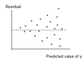$y$ Which of the following assumptions appears violated based on this plot?

In any production process in which one or more workers are engaged in a variety of tasks, the total time spent in production varies as a function of the size of the workpool and the level of output of the various activities. In a large metropolitan department store, it is believed that the number of man-hours worked $( y )$ per day by the clerical staff depends on the number of pieces of mail processed per day $\left( x _ { 1 } \right)$ and the number of checks cashed per day $\left( x _ { 2 } \right)$ . Data collected for $n = 20$ working days were used to fit the model: $E ( y ) = \beta _ { 0 } + \beta _ { 1 } x _ { 1 } + \beta _ { 2 } x _ { 2 }$ A partial printout for the analysis follows: Actual Predict Lower 95\% CL Upper 95\% CL OBS X1 X2 Value Value Residual Predict Predict 1 7781 644 74.707 83.175 -8.468 47.224 119.126 Interpret the 95% prediction interval for y shown on the printout.

If when using the model $E ( y ) = \beta _ { 0 } + \beta _ { 1 } x _ { 1 } + \beta _ { 2 } x _ { 2 } + \beta _ { 3 } x _ { 1 } x _ { 2 }$ we determine that interaction between and $x _ { 2 }$ is not significant, we can drop the $x _ { 1 } x _ { 2 }$ term from the model and use the simpler model $E ( y ) = \beta _ { 0 } + \beta _ { 1 } x _ { 1 } + \beta _ { 2 } x _ { 2 }$ .

When modeling E(y) with a single qualitative independent variable, the number $0 - 1$ dummy variables in the model is equal to the number of levels of the qualitative variable.

It is safe to conduct $t$ -tests on the individual $\beta$ parameters in a first-order linear model in order to determine which independent variables are useful for predicting $y$ and which are not.

We expect all or almost all of the residuals to fall within 2 standard deviations of 0.

The table shows the profit y (in thousands of dollars) that a company made during a month when the price of its product was x dollars per unit. Profit, y Price, x 12 1.20 17 1.25 20 1.29 21 1.30 24 1.35 26 1.39 27 1.40 23 1.45 21 1.49 20 1.50 15 1.55 11 1.59 10 1.60 5 1.65 a. Fit the model $y = \beta _ { 0 } + \beta _ { 1 } x + \beta _ { 2 } x 2 + \varepsilon$ to the data and give the least squares prediction equation. b. Plot the fitted equation on a scattergram of the data. c. Is there sufficient evidence of downward curvature in the relationship between profit and price? Use $\alpha = .05$ .