Exam 12: Multiple Regression and Model Building

In Hawaii, proceedings are under way to enable private citizens to own the property that their homes are built on. In prior years, only estates were permitted to own land, and homeowners leased the land from the estate. In order to comply with the new law, a large Hawaiian estate wants to use regression analysis to estimate the fair market value of the land. The following variables are proposed: $y = \text { Sale price of property (\$ thousands) }$ $x _ { 2 } = 1$ if property near Cove, 0 if not Write a regression model relating the sale price of a property to the qualitative variable x. Interpret all the ?s in the model.

It is desired to build a regression model to predict $\mathrm { y } =$ the sales price of a single family home, based. on the $x _ { 1 } =$ size of the house and $x _ { 2 } =$ the neighborhood the home is located in. The goal is to compare the prices of homes that are located in two different neighborhoods. The following complete 2 nd-order model is proposed: $\mathrm { E } ( \mathrm { y } ) = \beta _ { 0 } + \beta _ { 1 } \mathrm { x } _ { 1 } + \beta _ { 2 } \mathrm { x } _ { 1 } ^ { 2 } + \beta _ { 3 } \mathrm { x } _ { 2 } + \beta _ { 4 } \mathrm { x } _ { 1 } \mathrm { x } _ { 2 } + \beta _ { 5 } \mathrm { x } _ { 1 } ^ { 2 } \mathrm { x } _ { 2 }$ What hypothesis should be tested to determine if the quadratic terms are necessary to predict the sales price of a home?

As part of a study at a large university, data were collected on $n = 224$ freshmen computer science (CS) majors in a particular year. The researchers were interested in modeling $y$ , a student's grade point average (GPA) after three semesters, as a function of the following independent variables (recorded at the time the students enrolled in the university): $x _ { 1 } =$ average high school grade in mathematics (HSM) $x _ { 2 } =$ average high school grade in science (HSS) $x _ { 3 } =$ average high school grade in English (HSE) $x _ { 4 } =$ SAT mathematics score (SATM) $x _ { 5 } =$ SAT verbal score (SATV) A first-order model was fit to the data with the following results: SOURCE DF SS MS F VALUE PROB > F MODEL 5 28.64 5.73 11.69 .0001 ERROR 218 106.82 0.49 TOTAL 223 135.46 ROOT MSE 0.700 R-SQUARE 0.211 DEP MEAN 4.635 ADJ R-SQ 0.193 PARAMETER STANDARD T FOR 0: VARIABLE ESTIMATE ERROR PARAMETER = 0 PROB > |T| INTERCEPT 2.327 0.039 5.817 0.0001 X1 (HSM) 0.146 0.037 3.718 0.0003 X2 (HSS) 0.036 0.038 0.950 0.3432 X3 (HSE) 0.055 0.040 1.397 0.1637 X4 (SATM) 0.00094 0.00068 1.376 0.1702 X5 (SATV) -0.00041 0.0059 -0.689 0.4915 Test to determine if the model is adequate for predicting GPA. Use \alpha=.01 .

A study of the top MBA programs attempted to predict $y =$ the average starting salary (in $\$ 1000$ 's) of graduates of the program based on $x =$ the amount of tuition (in $\$ 1000$ 's) charged by the program. After first considering a simple linear model, it was decided that a quadratic model should be proposed. Which of the following models proposes a 2nd-order quadratic relationship between $x$ and $y$ ?

The printout shows the results of a first-order regression analysis relating the sales price $y$ of a product to the time in hours $x _ { 1 }$ and the cost of raw materials $x _ { 2 }$ needed to make the product. SUMMARY OUTPUT Regression Statistics Multiple R 0.997578302 R Square 0.995162468 Adjusted R Square 0.990324936 Standard Error 1.185250723 Observations 5 ANOVA df SS MS F Significance F Regression 2 577.9903614 288.9952 205.717 0.004837532 Residual 2 2.809638554 1.404819 Total 4 580.8 Coefficients Standard Error t Stat P -value Lower 95\% Upper 95\% Intercept -26.48433735 3.674668773 -7.20727 0.018713 -42.29517198 -10.67350271 Time -2.168674699 4.11406532 -0.52714 0.650732 -19.8700814 15.532732 Materials 8.142168675 1.094681583 7.437933 0.0176 3.432130693 12.85220666 a. What is the least squares prediction equation? b. Identify the SSE from the printout. c. Find the estimator of $\sigma ^ { 2 }$ for the model.

Stepwise regression is used to determine which variables, from a large group of variables, are useful in predicting the value of a dependent variable.

During its manufacture, a product is subjected to four different tests in sequential order. An efficiency expert claims that the fourth (and last) test is unnecessary since its results can be predicted based on the first three tests. To test this claim, multiple regression will be used to model Test4 score $( y )$ , as a function of Test1 score $\left( x _ { 1 } \right)$ , Test 2 score $\left( x _ { 2 } \right)$ , and Test3 score $\left( x _ { 3 } \right)$ . [Note: All test scores range from 200 to 800 , with higher scores indicative of a higher quality product.] Consider the model: $E ( y ) = \beta _ { 1 } + \beta _ { 1 } x _ { 1 } + \beta _ { 2 } x _ { 2 } + \beta _ { 3 } x _ { 3 }$ The first-order model was fit to the data for each of 12 units sampled from the production line. The results are summarized in the printout. SOURCE DF SS MS F VALUE PROB > F MODEL 3 151417 50472 18.16 .0075 ERROR 8 22231 2779 TOTAL 12 173648 ROOT MSE 52.72 R-SQUARE 0.872 DEP MEAN 645.8 ADJ R-SQ 0.824 PARAMETER STANDARD T FOR 0: VARIABLE ESTIMATE ERROR PARAMETER =0 PROB > || INTERCEPT 11.98 80.50 0.15 0.885 X1(TEST1) 0.2745 0.1111 2.47 0.039 X2(TEST2) 0.3762 0.0986 3.82 0.005 X3(TEST3) 0.3265 0.0808 4.04 0.004 Suppose the $95 \%$ confidence interval for $\beta _ { 3 }$ is $( .15 , .47 )$ . Which of the following statements is incorrect?

In any production process in which one or more workers are engaged in a variety of tasks, the total time spent in production varies as a function of the size of the workpool and the level of output of the various activities. In a large metropolitan department store, it is believed that the number of man-hours worked $( y )$ per day by the clerical staff depends on the number of pieces of mail processed per day $\left( x _ { 1 } \right)$ and the number of checks cashed per day $\left( x _ { 2 } \right)$ . Data collected for $n = 20$ working days were used to fit the model: $E ( y ) = \beta _ { 0 } + \beta _ { 1 } x _ { 1 } + \beta _ { 2 } x _ { 2 }$ A printout for the analysis follows: Analysis of Variance SOURCE DF SS MS F VALUE PROB > F MODEL 2 7089.06512 3544.53256 13.267 0.0003 ERROR 17 4541.72142 267.16008 C TOTAL 19 11630.78654 ROOT MSE 16.34503 R-SQUARE 0.6095 DEP MEAN 93.92682 ADJR-SQ 0.5636 C.V. 17.40188 Parameter Estimates PARAMETER STANDARD T FOR 0: VARIABLE DF ESTIMATE ERROR PARAMETER $=0 \quad$ PROB $>|\mathrm{T}|$ INTERCEPT 1 114.420972 18.68485744 6.124 0.0001 X1 1 -0.007102 0.00171375 -4.144 0.0007 X2 1 0.037290 0.02043937 1.824 0.0857 Actual Predict Lower 95\% CL Upper 95\% CL OBS 1 2 Value Value Residual Predict Predict 1 7781 644 74.707 83.175 -8.468 47.224 119.126 Test to determine if there is a positive linear relationship between the number of man-hours worked, $y$ , and the number of checks cashed per day, $x _ { 2 }$ . Use $\alpha = .05$ .

A collector of grandfather clocks believes that the price received for the clocks at an auction increases with the number of bidders, but at an increasing (rather than a constant) rate. Thus, the model proposed to best explain auction price (y, in dollars) by number of bidders (x) is the quadratic model $E ( y ) = \beta _ { 0 } + \beta _ { 1 } x + \beta _ { 2 } x ^ { 2 }$ This model was fit to data collected for a sample of 32 clocks sold at auction; the resulting estimate of $\beta _ { 1 }$ was $- .31$ . Interpret this estimate of $\beta _ { 1 }$ .

A study of the top MBA programs attempted to predict the average starting salary (in $1000's) of graduates of the program based on the amount of tuition (in $1000's) charged by the program and the average GMAT score of the program's students. The results of a regression analysis based on a sample of 75 MBA programs is shown below: $\text { Least Squares Linear Regression of Salary }$ Predictor Variables Coefficient Std Error T P VIF Constant -203.402 51.6573 -3.94 0.0002 0.0 Gmat 0.39412 0.09039 4.36 0.0000 2.0 Tuition 0.92012 0.17875 5.15 0.0000 2.0 R-Squared 0.6857 Resid. Mean Square (MSE) 427.511 Adjusted R-Squared 0.6769 Standard Deviation 20.6763 Interpret the coefficient for the tuition variable shown on the printout.

As part of a study at a large university, data were collected on $n = 224$ freshmen computer science (CS) majors in a particular year. The researchers were interested in modeling $y$ , a student's grade point average (GPA) after three semesters, as a function of the following independent variables (recorded at the time the students enrolled in the university): $x _ { 1 } =$ average high school grade in mathe $x _ { 2 } =$ average high school grade in scien $x _ { 3 } =$ average high school grade in Eng $x _ { 4 } =$ SAT mathematics score (SATM) $x _ { 5 } =$ SAT verbal score (SATV) A first-order model was fit to data. Give the null hypothesis for testing the overall adequacy of the model.

A collector of grandfather clocks believes that the price received for the clocks at an auction increases with the number of bidders, but at an increasing (rather than a constant) rate. Thus, the model proposed to best explain auction price ( $y$ , in dollars) by number of bidders $( x )$ is the quadratic model $E ( y ) = \beta _ { 0 } + \beta _ { 1 } x + \beta _ { 2 } x ^ { 2 }$ This model was fit to data collected for a sample of 32 clocks sold at auction; a portion of the printout follows: PARAMETER STANDARD TFOR 0 : VARIABLES ESTIMATE ERROR PARAMETER =0 PROB >|| INTERCEPT 286.42 9.66 29.64 .0001 X -.31 .06 -5.14 .0016 \cdot .000067 .00007 .95 .3600 Find the $p$ -value for testing $H _ { 0 } : \beta _ { 2 } = 0$ against $H _ { \mathrm { a } } : \beta _ { 2 } > 0$ .

An elections officer wants to model voter turnout $( y )$ in a precinct as a function of the type of precinct. Consider the model relating mean voter turnout, $E ( y )$ , to precinct type: E(y)=++, where =1 if urban, 0 if not =1 if suburban, 0 if not (Base level = rural) Interpret the value of $\beta _ { 0 }$ .

It is desired to build a regression model to predict $\mathrm { y } =$ the sales price of a single family home, based on the $x _ { 1 } =$ size of the house and $x _ { 2 } =$ the neighborhood the home is located in. The goal is to compare the prices of homes that are located in two different neighborhoods. A complete 2nd-order model is proposed. Which regression model proposes the complete 2 nd-order model?

Residual analysis can be used to check for violations of the assumptions that the distribution of the random error component is normally distributed with mean 0.

Retail price data for $n = 60$ hard disk drives were recently reported in a computer magazine. Three variables were recorded for each hard disk drive: $y =$ Retail PRICE (measured in dollars) $x _ { 1 } =$ Microprocessor SPEED (measured in megahertz) (Values in sample range from 10 to 40 ) $x _ { 2 } =$ CHIP size (measured in computer processing units) (Values in sample range from 286 to 486 ) a first-order regression model was fit to the data. Part of the printout follows: Dep Var Predict Std Err Lower 95\% Upper 95\% OBS SPEED CHIP PRICE Value Predict Predict Predict Residual 1 33 286 5099.0 4464.9 260.768 3942.7 4987.1 634.1 Interpret the interval given in the printout.

The model $E ( y ) = \beta _ { 0 } + \beta _ { 1 } x$ was fit to a set of data, and the following plot of residuals against $x$ values was obtained. 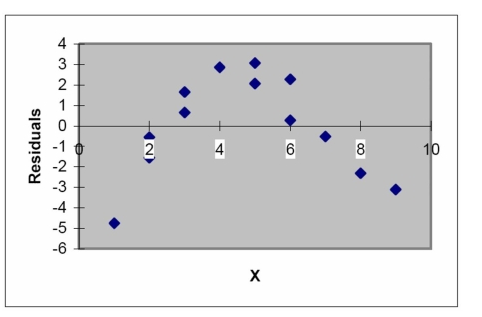Interpret the residual plot.

The stepwise regression model should not be used as the final model for predicting y.

A first-order model does not contain any higher-order terms.

In any production process in which one or more workers are engaged in a variety of tasks, the total time spent in production varies as a function of the size of the workpool and the level of output of the various activities. In a large metropolitan department store, it is believed that the number of man-hours worked $( y )$ per day by the clerical staff depends on the number of pieces of mail processed per day $\left( x _ { 1 } \right)$ and the number of checks cashed per day $\left( x _ { 2 } \right)$ . Data collected for $n = 20$ working days were used to fit the model: $E ( y ) = \beta _ { 0 } + \beta _ { 1 } x _ { 1 } + \beta _ { 2 } x _ { 2 }$ A partial printout for the analysis follows: $\quad$$\quad$$\quad$$\quad$$\quad$$\quad$$\quad$$\quad$$\quad$$\quad$$\quad$$\quad$$\quad$$\quad$$\text{Parameter Estimates}$ PARAMETER STANDARD T FOR 0: VARIABLE DF ESTIMATE ERROR PARAMETER = 0 PROB > |T| INTERCEPT 1 114.420972 18.6848744 6.124 0.0001 X1 1 -0.007102 0.00171375 -4.144 0.0007 X2 1 0.037290 0.02043937 1.824 0.0857 Calculate a $95 \%$ confidence interval for $\beta _ { 1 }$ .