Exam 12: Multiple Regression and Model Building

As part of a study at a large university, data were collected on $n = 224$ freshmen computer science (CS) majors in a particular year. The researchers were interested in modeling $y$ , a student's grade point average (GPA) after three semesters, as a function of the following independent variables (recorded at the time the students enrolled in the university): $x _ { 1 } =$ average high school grade in mathematics (HSM) $x _ { 2 } =$ average high school grade in science (HSS) $x _ { 3 } =$ average high school grade in English (HSE) $x _ { 4 } =$ SAT mathematics score (SATM) $x _ { 5 } =$ SAT verbal score (SATV) A first-order model was fit to data with $R ^ { 2 } = 0.211$ . What is the correct interpretation of $R ^ { 2 }$ , the coefficient of determination for the model?

When using the model $E ( y ) = \beta _ { 0 } + \beta _ { 1 } x$ for one qualitative independent variable with a $0 - 1$ coding convention, $\beta _ { 1 }$ represents the difference between the mean responses for the level assigned the value 1 and the base level.

A study of the top MBA programs attempted to predict the average starting salary (in $1000's) of graduates of the program based on the amount of tuition (in $1000's) charged by the program and The average GMAT score of the program's students. The results of a regression analysis based on a Sample of 75 MBA programs is shown below: Least Squares Linear Regression of Salary The model was then used to create 95% confidence and prediction intervals for y and for E(Y) when The tuition charged by the MBA program was $75,000 and the GMAT score was 675. The results are Shown here: 95% confidence interval for E(Y): ($126,610, $136,640) 95% prediction interval for Y: ($90,113, $173,160) Which of the following interpretations is correct if you want to use the model to estimate E(Y) for All MBA programs?

A college admissions officer proposes to use regression to model a student's college GPA at graduation in terms of the following two variables: = high school GPA = SAT score The admissions officer believes the relationship between college GPA and high school GPA is linear and the relationship between SAT score and college GPA is linear. She also believes that the relationship between college GPA and high school GPA depends on the student's SAT score. She proposes the regression model: $E ( y ) = \beta _ { 0 } + \beta _ { 1 } x _ { 1 } + \beta _ { 2 } x _ { 2 } + \beta _ { 3 } x _ { 1 } x _ { 2 }$ Explain how to determine if the relationship between college GPA and SAT score depends on the high school GPA.

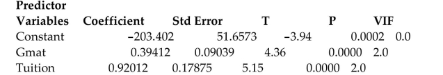
A study of the top MBA programs attempted to predict the average starting salary (in $1000's) of graduates of the program based on the amount of tuition (in $1000's) charged by the program and the average GMAT score of the program's students. The results of a regression analysis based on a sample of 75 MBA programs is shown below: Least Squares Linear Regression of Salary Predictor Variables Coefficient Std Error T P VIF Constant -203.402 51.6573 -3.94 0.0002 0.0 Gmat 0.39412 0.09039 4.36 0.0000 2.0 Tuition 0.92012 0.17875 5.15 0.0000 2.0 Source DF SS MS F P Regression 2 67140.9 33570.5 78.53 0.0000 Residual 72 30780.8 427.5 Total 74 97921.7 Interpret the p-value for the global f-test shown on the printout.

A term that contains the value of a quantitative variable raised to the second power is called a higher-order term.

In the first-order model $E ( y ) = \beta _ { 0 } + \beta _ { 1 } x _ { 1 } + \beta _ { 2 } x _ { 2 } + \beta _ { 3 } x _ { 3 } , \beta _ { 2 }$ represents the slope of the line relating $y$ to $x _ { 2 }$ when $\beta _ { 1 }$ and $\beta _ { 3 }$ are both held fixed.

As part of a study at a large university, data were collected on $n = 224$ freshmen computer science (CS) majors in a particular year. The researchers were interested in modeling $y$ , a student's grade point average (GPA) after three semesters, as a function of the following independent variables (recorded at the time the students enrolled in the university): $x _ { 1 } =$ average high school grade in mathematics (HSM) $x _ { 2 } =$ average high school grade in science (HSS) $x _ { 3 } =$ average high school grade in English (HSE) $x _ { 4 } =$ SAT mathematics score (SATM) $x _ { 5 } =$ SAT verbal score (SATV) A first-order model was fit to data with $R _ { a } ^ { 2 } = .193$ . Interpret the value of the adjusted coefficient of determination $R _ { a } ^ { 2 }$ .

When testing the utility of the quadratic model $E ( y ) = \beta _ { 0 } + \beta _ { 1 } x + \beta _ { 2 } x ^ { 2 }$ , the most important tests involve the null hypotheses $H _ { 0 } : \beta _ { 0 } = 0$ and $H _ { 0 } : \beta _ { 1 } = 0$ .

The model $E ( y ) = \beta _ { 0 } + \beta _ { 1 } x$ was fit to a set of data, and the following plot of residuals against $x$ values was obtained. 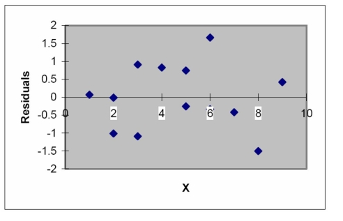Interpret the residual plot.

A collector of grandfather clocks believes that the price received for the clocks at an auction increases with the number of bidders, but at an increasing (rather than a constant) rate. Thus, the model proposed to best explain auction price ( $y$ , in dollars) by number of bidders $( x )$ is the quadratic model $E ( y ) = \beta _ { 0 } + \beta _ { 1 } x + \beta _ { 2 } x ^ { 2 }$ This model was fit to data collected for a sample of 32 clocks sold at auction; a portion of the printout follows: PARAMETER STANDARD T FOR 0: VARIABLES ESTIMATE ERROR PARAMETER =0 PROB > |T| INTERCEPT 286.42 9.66 29.64 .0001 .31 .06 5.14 .0016 \cdot -.000067 .00007 -0.95 .3600 Give the $p$ -value for testing $H _ { 0 } : \beta _ { 2 } = 0$ against $H _ { \mathrm { a } } : \beta _ { 2 } \neq 0$ .

Consider the partial printout below. Coefficients Standard Error t Stat P-value Lower 95\% Upper 95\% Intercept -63.14873931 25.09115112 -2.516773304 0.045484943 -124.5446192 -1.752859365 14.72507864 8.113581741 1.814867849 0.119466699 -5.128155197 34.57831248 X2 12.48784546 4.686063743 2.664890224 0.037279879 1.021452165 23.95423875 X1X2 -1.886935135 1.344999834 -1.402925924 0.210210141 -5.178033575 1.404163305 Is there evidence (at \alpha=.05 ) that and interact? Explain.

Which of the following is not a possible indicator of multicollinearity?

In regression, it is desired to predict the dependent variable based on values of other related independent variables. Occasionally, there are relationships that exist between the independent variables. Which of the following multiple regression pitfalls does this example describe?

The first-order model below was fit to a set of data. $E ( y ) = \beta _ { 0 } + \beta _ { 1 } x _ { 1 } + \beta _ { 2 } x _ { 2 }$ Explain how to determine if the constant variance assumption is satisfied.

A study of the top MBA programs attempted to predict the average starting salary (in $1000's) of graduates of the program based on the amount of tuition (in $1000's) charged by the program and the average GMAT score of the program's students. The results of a regression analysis based on a sample of 75 MBA programs is shown below: Least Squares Linear Regression of Salary Predictor Variables Coefficient Std Error T P \multicolumn 2 c VIF Constant -203.402 51.6573 -3.94 0.0002 0.0 Gmat 0.39412 0.09039 4.36 0.0000 2.0 Tuition 0.92012 0.17875 5.15 0.0000 2.0 The model was then used to create 95% confidence and prediction intervals for y and for E(Y) when the tuition charged by the MBA program was $75,000 and the GMAT score was 675. The results are shown here: 95% confidence interval for E(Y): ($126,610, $136,640) 95% prediction interval for Y: ($90,113, $173,160) Which of the following interpretations is correct if you want to use the model to estimate Y for a single MBA program?

Which residual plot would you examine to determine whether the assumption of constant error variance is satisfied for a model with two independent variables $x _ { 1 }$ and $x _ { 2 }$ ?

Which equation represents a complete second-order model for two quantitative independent variables?

Probabilistic models that include more than one dependent variable are called multiple regression models.

Consider the model $y = \beta _ { 0 } + \beta _ { 1 } x _ { 1 } + \beta _ { 2 } x _ { 2 } + \beta _ { 3 } x _ { 3 } + \varepsilon$ where $x _ { 1 }$ is a quantitative variable and $x _ { 2 }$ and $x _ { 3 }$ are dummy variables describing a qualitative variable at three levels using the coding scheme $x _ { 2 } = \left\{ \begin{array} { l l } 1 & \text { if level } 2 \\ 0 & \text { otherwise } \end{array} \quad x _ { 3 } = \left\{ \begin{array} { l l } 1 & \text { if level } 3 \\ 0 & \text { otherwise } \end{array} \right. \right.$ The resulting least squares prediction equation is $\hat { y } = 16.3 + 2.3 x _ { 1 } + 3.5 x _ { 2 } + 18 x _ { 3 }$ . What is the response line (equation) for $E ( y )$ when $x _ { 2 } = 0$ and $x _ { 3 } = 1$ ?