Question 1

Why is the random error term ? added to a multiple regression model?

Accepted Answer

The random error ter

Question 2

Retail price data for $n = 60$ hard disk drives were recently reported in a computer magazine. Three variables were recorded for each hard disk drive:
$y =$ Retail PRICE (measured in dollars)
$x _ { 1 } =$ Microprocessor SPEED (measured in megahertz)
(Values in sample range from 10 to 40 )
$x _ { 2 } =$ CHIP size (measured in computer processing units)
(Values in sample range from 286 to 486 )

A first-order regression model was fit to the data. Part of the printout follows:
$\begin{array}{lrrrrr} 
& {\text { Analysis of Variance }} \
\text { SOURCE } & \text { DF } & \text { SS } & \text { MS } & \text { F VALUE } & \text { PROB > F } \
\text { MODEL } & 2 & 34593103.008 & 17296051.504 & 19.018 & 0.0001 \
\text { ERROR } & 57 & 51840202.926 & 909477.24431 & & \
\text { CTOTAL } & 59 & 86432305.933 & & &
\end{array}$

$\begin{array}{llll}
\text { ROOT MSE } & 953.66516 & \text { R-SQUARE } & 0.4002 \
\text { DEP MEAN } & 3197.96667 & \text { ADJ R-SQ } & 0.3792 \
\text { C.V. } & 29.82099 & &
\end{array}$

Test to determine if the model is adequate for predicting the price of a computer. Use $\alpha =$ $.01$.

Accepted Answer

To determine if the model is useful for

Question 3

A qualitative variable whose outcomes are assigned numerical values is called a coded variable.

Accepted Answer

A) True 
 B)False

Question 4

The stepwise regression procedure may not be used when the inclusion of one or more dummy variables is under consideration.

Accepted Answer

A) True 
 B)False

Question 5

Consider the interaction model $E ( y ) = 3.6 + 1.2 x _ { 1 } + 2.4 x _ { 2 } + .2 x _ { 1 } x _ { 2 }$. Determine the change in $E ( y )$ when $x _ { 1 }$ is changed from 6 to 7 and $x _ { 2 }$ is held fixed at 3 .

Accepted Answer

A)  4.2 
B)  10.8 
C)  11.4 
D)  1.8 
A)  4.2 
B)  10.8 
C)  11.4 
D)  1.8

Question 6

As part of a study at a large university, data were collected on $n = 224$ freshmen computer science (CS) majors in a particular year. The researchers were interested in modeling $y$, a student's grade point average (GPA) after three semesters, as a function of the following independent variables (recorded at the time the students enrolled in the university):
$x _ { 1 } =$ average high school grade in mathematics (HSM)
$x _ { 2 } =$ average high school grade in science (HSS)
$x _ { 3 } =$ average high school grade in English (HSE)
$x _ { 4 } =$ SAT mathematics score (SATM)
$x _ { 5 } =$ SAT verbal score (SATV)

A first-order model was fit to data.

A $95 \%$ confidence interval for $\beta _ { 1 }$ is $( .06 , .22 )$. Interpret this result.

Accepted Answer

A)  $95 \%$ of the GPAs fall within .06 to $.22$ of their true values. 
B)  We are $95 \%$ confident that a CS freshman's HS math grade increases by an amount between $.06$ and $.22$ for every 1-point increase in GPA, holding $x _ { 2 } - x _ { 5 }$ constant. 
C)  We are $95 \%$ confident that the mean GPA of all CS freshmen after three semesters falls between 06 and .22. 
D)  We are $95 \%$ confident that a CS freshman's GPA increases by an amount between .06 and .22 for every 1-point increase in average HS math grade, holding $x _ { 2 } - x _ { 5 }$ constant. 
A)  $95 \%$ of the GPAs fall within .06 to $.22$ of their true values. 
B)  We are $95 \%$ confident that a CS freshman's HS math grade increases by an amount between $.06$ and $.22$ for every 1-point increase in GPA, holding $x _ { 2 } - x _ { 5 }$ constant. 
C)  We are $95 \%$ confident that the mean GPA of all CS freshmen after three semesters falls between 06 and .22. 
D)  We are $95 \%$ confident that a CS freshman's GPA increases by an amount between .06 and .22 for every 1-point increase in average HS math grade, holding $x _ { 2 } - x _ { 5 }$ constant.

Question 7

A graphing calculator was used to fit the model $E ( y ) = \beta _ { 0 } + \beta _ { 1 } x + \beta _ { 2 } x ^ { 2 }$ to a set of data. The resulting screen is shown below.

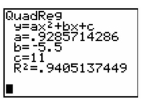Which number on the screen represents the estimator of $\beta _ { 2 }$ ?

Accepted Answer

A)  11 
B)  .9286 
C)  5.5 
D)  .9405 
A)  11 
B)  .9286 
C)  5.5 
D)  .9405

Question 8

Consider the model
$$y = \beta _ { 0 } + \beta _ { 1 } x _ { 1 } + \beta _ { 2 } x _ { 1 } ^ { 2 } + \beta _ { 3 } x _ { 2 } + \beta _ { 4 } x _ { 3 } + \beta _ { 5 } x _ { 1 } x _ { 2 } + \beta _ { 6 } x _ { 1 } x _ { 3 } + \beta _ { 7 } x _ { 1 } 2 _ { x _ { 2 } } + \beta _ { 8 } x _ { 1 } x _ { 3 } + \varepsilon$$
where $x _ { 1 }$ is a quantitative variable and $x _ { 2 }$ and $x _ { 3 }$ are dummy variables describing a qualitative variable at three levels using the coding scheme
$$x _ { 2 } = \left\{ \begin{array} { l l } 
1 & \text { if level } 2 \
0 & \text { otherwise }
\end{array} \quad x _ { 3 } = \left\{ \begin{array} { l l } 
1 & \text { if level } 3 \
0 & \text { otherwise }
\end{array} \right. \right.$$
The resulting least squares prediction equation is
$$\hat { y } = 8.8 - 1.1 x _ { 1 } + 3.2 x _ { 1 } ^ { 2 } + 1.6 x _ { 2 } - 4.4 x _ { 3 } + .02 x _ { 1 } x _ { 2 } + 1.3 x _ { 1 } x _ { 3 } + .01 x _ { 1 } 2 ^ { 2 } - .06 x _ { 1 } x _ { 3 }$$
What is the equation of the response curve for $E ( y )$ when $x _ { 2 } = 0$ and $x _ { 3 } = 0$ ?

Accepted Answer

A)  $\hat { y } = 8.8 - 1.1 x _ { 1 } + 3.2 x _ { 1 } { } ^ { 2 }$ 
B)  $\hat { y } = 8.8 - 1.3 x _ { 1 } + 3.2 x _ { 1 } ^ { 2 }$ 
C)  $\hat { y } = 8.8 - 1.6 x _ { 2 } - 4.4 x _ { 3 }$ 
D)  $\hat { y } = 8.8 - .22 x _ { 1 } + 3.15 x _ { 1 } 2$ 
A)  $\hat { y } = 8.8 - 1.1 x _ { 1 } + 3.2 x _ { 1 } { } ^ { 2 }$ 
B)  $\hat { y } = 8.8 - 1.3 x _ { 1 } + 3.2 x _ { 1 } ^ { 2 }$ 
C)  $\hat { y } = 8.8 - 1.6 x _ { 2 } - 4.4 x _ { 3 }$ 
D)  $\hat { y } = 8.8 - .22 x _ { 1 } + 3.15 x _ { 1 } 2$

Question 9

For any given model fit to a data set, the sum of the residuals is 0.

Accepted Answer

A) True 
 B)False

Question 10

The method of fitting first-order models is the same as that of fitting the simple straight-line model, i.e. the method of least squares.

Accepted Answer

A) True 
 B)False

Question 11

During its manufacture, a product is subjected to four different tests in sequential order. An efficiency expert claims that the fourth (and last) test is unnecessary since its results can be predicted based on the first three tests. To test this claim, multiple regression will be used to model Test4 score $( y )$, as a function of Test1 score $\left( x _ { 1 } \right)$, Test 2 score $\left( x _ { 2 } \right)$, and Test3 score $\left( x _ { 3 } \right)$. [Note: All test scores range from 200 to 800 , with higher scores indicative of a higher quality product.] Consider the model:
$$E ( y ) = \beta _ { 1 } + \beta _ { 1 } x _ { 1 } + \beta _ { 2 } x _ { 2 } + \beta _ { 3 } x _ { 3 }$$
The first-order model was fit to the data for each of 12 units sampled from the production line.
A $95 \%$ prediction interval for Test4 score of a product with Test1 $= 590$, Test2 $= 750$, and Test $3 = 710$ is $( 583,793 )$. Interpret this result.

Accepted Answer

A)  We are $95 \%$ confident that a product's Test 4 score will fall between 583 and 793 points when the first three scores are 590,750 , and 710 , respectively. 
B)  Since 0 is outside the interval, there is evidence of a linear relationship between Test4 score and any of the other test scores. 
C)  We are $95 \%$ confident that the mean Test4 score of all manufactured products falls between 583 and 793 points. 
D)  We are $95 \%$ confident that a product's Test 4 score increases by an amount between 583 and 793 points for every 1 point increase in Test1 score, holding Test 2 and Test 3 score constant. 
A)  We are $95 \%$ confident that a product's Test 4 score will fall between 583 and 793 points when the first three scores are 590,750 , and 710 , respectively. 
B)  Since 0 is outside the interval, there is evidence of a linear relationship between Test4 score and any of the other test scores. 
C)  We are $95 \%$ confident that the mean Test4 score of all manufactured products falls between 583 and 793 points. 
D)  We are $95 \%$ confident that a product's Test 4 score increases by an amount between 583 and 793 points for every 1 point increase in Test1 score, holding Test 2 and Test 3 score constant.

Question 12

The staff of a test kitchen is attempting to determine the baking time, $y$, of a roast, i.e., the time it takes the internal temperature of the roast to reach $165 ^ { \circ } \mathrm { F }$, using two variables, the temperature setting of the oven, $x _ { 1 }$, and the weight of the roast, $x _ { 2 }$, in pounds. The data for 24 roasts are shown below.
Baking Times of Roasts
$\begin{array}{lll|lll|lll|lll|lll|lll}
\mathrm{X} 1\left({ }^{\circ} \mathrm{F}\right) & \mathrm{X} 2(\mathrm{lb}) & \mathrm{Y}(\mathrm{hr}) & \mathrm{X} 1\left({ }^{\circ} \mathrm{F}\right) & \mathrm{X} 2(\mathrm{lb}) & \mathrm{Y}(\mathrm{hr}) & \mathrm{X} 1\left({ }^{\circ} \mathrm{F}\right) & \mathrm{X} 2(\mathrm{lb})&\mathrm{Y}(\mathrm{hr}) & \mathrm{X} 1\left({ }^{\circ} \mathrm{F}\right) & \mathrm{X} 2(\mathrm{lb}) &\mathrm{Y}(\mathrm{hr}) \
\hline 300 & 2.2 & 2.6 & 325 & 2.1 & 2.3 & 350 & 2.3 & 2.2 & 375 & 2.2 & 1.9 \
300 & 2.7 & 2.8 & 325 & 2.4 & 2.4 & 350 & 2.5 & 2.3 & 375 & 2.6 & 2.2 \
300 & 2.9 & 3.1 & 325 & 2.9 & 2.6 & 350 & 2.8 & 2.5 & 375 & 2.9 & 2.4 \
300 & 3.1 & 3.2 & 325 & 3.0 & 2.7 & 350 & 3.2 & 2.7 & 375 & 3.1 & 2.6 \
300 & 3.2 & 3.2 & 325 & 3.2 & 2.9 & 350 & 3.4 & 2.8 & 375 & 3.3 & 2.7 \
300 & 3.5 & 3.3 & 325 & 3.6 & 3.1 & 350 & 3.5 & 2.8 & 375 & 3.4 & 2.7 \
\hline
\end{array}$

a. Fit a complete second-order model to the data.
b. Do the data provide sufficient evidence to indicate that the second-order terms contribute information for the prediction of $y$ ? State the null and alternative hypotheses and the test statistic. Use $\alpha = .05$.

Accepted Answer

a. @#LAT-DLM&
b. @#LAT-DLM&
@#LAT-DLM& At least one of the parameters

Question 13

One of three surfaces is produced by a complete second-order model with two quantitative independent variables: a paraboloid that opens upward, a paraboloid that opens downward, or a saddle-shaped surface.

Accepted Answer

A) True 
 B)False

Question 14

There are four independent variables, $x _ { 1 } , x _ { 2 } , x _ { 3 }$, and $x _ { 4 }$, that might be useful in predicting a response $y$. A total of $n = 40$ observations is available, and it is decided to employ stepwise regression to help in selecting the independent variables that appear to useful. The computer fits all possible one-variable models of the form $E ( y ) = \beta _ { 0 } + \beta _ { 1 } x _ { i } , i = 1,2,3,4$. The information in the table is provided from the computer printout.
$\begin{array}{lrr}
\hline \text { Variable } &{\beta} &{s} \
\hline \mathrm{X} 1 & 2.4 & 0.52 \
\mathrm{X} 2 & -0.2 & 0.03 \
\mathrm{X} 3 & 3.6 & 2.11 \
\mathrm{X} 4 & 0.8 & 0.44 \
\hline
\end{array}$

Which independent variable is declared the best one-variable predictor of $y$ ?

Accepted Answer

A)  $x _ { 1 }$ 
B)  $x _ { 2 }$ 
C)  $x _ { 3 }$ 
D)  $x _ { 4 }$ 
A)  $x _ { 1 }$ 
B)  $x _ { 2 }$ 
C)  $x _ { 3 }$ 
D)  $x _ { 4 }$

Question 15

A public health researcher wants to use regression to predict the sun safety knowledge of pre-school children. The researcher randomly sampled 35 preschoolers, assigned them to one of Two groups, and then measured the following three variables: 
SUNSCORE: $\quad \mathrm { y } =$ Score on sun-safety comprehension test
READING: $\quad \mathrm { x } _ { 1 } =$ Reading comprehension score
GROUP: $\quad\quad x _ { 2 } = 1$ if child received a Be Sun Safe demonstration, 0 if not

The following two models were hypothesized:
Model 1: $E ( y ) = \beta _ { 0 } + \beta _ { 1 } x _ { 1 } + \beta _ { 2 } x _ { 1 } ^ { 2 } + \beta _ { 3 } x _ { 2 } + \beta _ { 4 } x _ { 1 } x _ { 2 } + \beta _ { 5 } x _ { 1 } ^ { 2 } x _ { 2 }$
Model 2: $E ( y ) = \beta _ { 0 } + \beta _ { 1 } x _ { 1 } + \beta _ { 3 } x _ { 2 } + \beta _ { 4 } x _ { 1 } x _ { 2 }$

A partial f-test was conducted to compare the two models and the resulting p-value was found to be 0.0023. Fill in the blank. The results lead us to conclude that there is _____$\text { (at } \alpha = 0.05 )$

Accepted Answer

A)  insufficient evidence of quadratic relationship between sun-safety score to reading score. 
B)  sufficient evidence of a statistically useful model for sun-safety score. 
C)  sufficient evidence of interaction between sun-safety score and reading score. 
D)  sufficient evidence of a quadratic relationship between sun-safety score to reading score. 
A)  insufficient evidence of quadratic relationship between sun-safety score to reading score. 
B)  sufficient evidence of a statistically useful model for sun-safety score. 
C)  sufficient evidence of interaction between sun-safety score and reading score. 
D)  sufficient evidence of a quadratic relationship between sun-safety score to reading score.

Question 16

We decide to conduct a multiple regression analysis to predict the attendance at a major league baseball game. We use the size of the stadium as a quantitative independent variable and the type Of game as a qualitative variable (with two levels - day game or night game). We hypothesize the
Following model: $$\mathrm { E } ( \mathrm { y } ) = \beta _ { 0 } + \beta _ { 1 ^ { \mathrm { x } } 1 } + \beta _ { 2 \mathrm { x } _ { 2 } } + \beta _ { 3 } \mathrm { x } _ { 3 }$$
Where$\quad $ $x _ { 1 } =$ size of the stadium 
$\quad $$\quad $$\quad $$x _ { 2 } = 1$ if a day game, 0 if a night game

A plot of the $y - x _ { 1 }$ relationship would show:

Accepted Answer

A)  Two non-parallel curves 
B)  Two parallel lines 
C)  Two parallel curves 
D)  Two non-parallel lines 
A)  Two non-parallel curves 
B)  Two parallel lines 
C)  Two parallel curves 
D)  Two non-parallel lines

Question 17

The model $E ( y ) = \beta _ { 0 } + \beta _ { 1 } x _ { 1 } + \beta _ { 2 } x _ { 2 }$ was fit to a set of data.
A partial printout for the analysis follows:
$\begin{array} { r r r r r r r r r } 
\hline & & & \text { Actual } & \text { Predict } & & \text { Lower 95\% CL } & \text { Upper 95\% CL } \
\text { OBS } & \text { X1 } & \text { X2 } & \text { Value } & \text { Value } & \text { Residual } & \text { Predict } & \text { Predict } \
1 & 7781 & 644 & 74.707 & 83.175 & - 8.468 & 47.224 & 119.126 \
\hline
\end{array}$

Interpret the value of the residual when $x _ { 1 } = 7,781$ and $x _ { 2 } = 644$.

Accepted Answer

A)  Since the residual is not 0 , the model is not useful for predicting $y$. 
B)  The predicted $\hat { y }$ is $8.468$ less than the observed value of $y$. 
C)  Since the residual is negative, there is evidence of a negative linear relationship between $y$ and at least one of the two independent variables. 
D)  The predicted $\hat { y }$ exceeds the observed value of $y$ by $8.468$. 
A)  Since the residual is not 0 , the model is not useful for predicting $y$. 
B)  The predicted $\hat { y }$ is $8.468$ less than the observed value of $y$. 
C)  Since the residual is negative, there is evidence of a negative linear relationship between $y$ and at least one of the two independent variables. 
D)  The predicted $\hat { y }$ exceeds the observed value of $y$ by $8.468$.

Question 18

An elections officer wants to model voter turnout $( y )$ in a precinct as a function of the type of precinct.
Consider the model relating mean voter turnout, $E ( y )$, to precinct type:
$$\begin{array} { l l } 
E ( y ) = \beta _ { 0 } + \beta _ { 1 } x _ { 1 } + \beta _ { 2 } x _ { 2 } , \text { where } & x _ { 1 } = 1 \text { if urban, } 0 \text { if not } \
& x _ { 2 } = 1 \text { if suburban, } 0 \text { if not } \
& \text { (Base level = rural) }
\end{array}$$
The $p$-value for the test $H _ { 0 } : \beta _ { 1 } = \beta _ { 2 } = 0$ is . 14 . Interpret the result.

Accepted Answer

A)  Reject $H _ { 0 }$ at $\alpha = .10$; the model is useful for predicting voter turnout. 
B)  Reject $H _ { 0 }$ at $\alpha = .01$; there is evidence of a difference between the mean voter turnouts for urban, suburban, and rural precincts. 
C)  Reject the model since it only explains $14 \%$ of the variation. 
D)  Do not reject $H _ { 0 }$ at $\alpha = .10$; there is no evidence of a difference between the mean voter turnouts for urban, suburban, and rural precincts. 
A)  Reject $H _ { 0 }$ at $\alpha = .10$; the model is useful for predicting voter turnout. 
B)  Reject $H _ { 0 }$ at $\alpha = .01$; there is evidence of a difference between the mean voter turnouts for urban, suburban, and rural precincts. 
C)  Reject the model since it only explains $14 \%$ of the variation. 
D)  Do not reject $H _ { 0 }$ at $\alpha = .10$; there is no evidence of a difference between the mean voter turnouts for urban, suburban, and rural precincts.

Question 19

A study of the top MBA programs attempted to predict the average starting salary (in $1000's) of graduates of the program based on the amount of tuition (in $1000's) charged by the program and the average GMAT score of the program's students. The results of a regression analysis based on a sample of 75 MBA programs is shown below: Least Squares Linear Regression of Salary
$\begin{array}{l}
\text { Predictor }\
\begin{array}{lccccccc}
\text { Variables } & \text { Coefficient } & \text { Std Error } & \text { T } & \text { P } & {\text { VIF }} \
\text { Constant } & -203.402 & 51.6573 & -3.94 & {0.0002} & 0.0 \
\text { Gmat } & 0.39412 & 0.09039 & 4.36 & 0.0000 & 2.0
\end{array}
\end{array}$

$\begin{array}{lrrr}
\text { R-Squared } & 0.6857 & \text { Resid. Mean Square (MSE) } & 427.511 \
\text { Adjusted R-Squared } & 0.6769 & \text { Standard Deviation } & 20.6763
\end{array}$

Identify the test statistic that should be used to test to determine if the amount of tuition charged by a program is a useful predictor of the average starting salary of the graduates of the program.

Accepted Answer

A)  $t = 5.15$ 
B)  $t = 20.67$ 
C)  $t = - 3.94$ 
D)  $t = 4.36$ 
A)  $t = 5.15$ 
B)  $t = 20.67$ 
C)  $t = - 3.94$ 
D)  $t = 4.36$

Question 20

As part of a study at a large university, data were collected on $n = 224$ freshmen computer science (CS) majors in a particular year. The researchers were interested in modeling $y$, a student's grade point average (GPA) after three semesters, as a function of the following independent variables (recorded at the time the students enrolled in the university):
$x _ { 1 } =$ average high school grade in mathematics (HSM)
$x _ { 2 } =$ average high school grade in science (HSS)
$x _ { 3 } =$ average high school grade in English (HSE)
$x _ { 4 } =$ SAT mathematics score (SATM)
$x _ { 5 } =$ SAT verbal score (SATV)

A first-order model was fit to data with the following results:

$\begin{array}{lrrrrr}
\hline \text { SOURCE } & \text { DF } & \text { SS } & \text { MS } & \text { F VALUE } & \text { PROB > F } \
\text { MODEL } & 5 & 28.64 & 5.73 & 11.69 & .0001 \
\text { ERROR } & 218 & 106.82 & 0.49 & & \
\text { TOTAL } & 223 & 135.46 & & &
\end{array}$

$\begin{array}{lccc}
\text { ROOT MSE } & 0.700 & \text { R-SQUARE } & 0.211 \
\text { DEP MEAN } & 4.635 & \text { ADJR-SQ } & 0.193
\end{array}$
 $\begin{array}{l}
\begin{array} { l r r r r } 
& \text {PARAMETER }& \text {STANDARD}& \text {T FOR 0:}\
 \text {VARIABLES}&\text { ESTIMATE } & \text { ERROR } & \text { PARAMETER } = 0 & \text { PROB } > | T |  \ 
\
\text { INTERCEPT } & 2.327 & 0.039 & 5.817 & 0.0001 \
\text { X1 (HSM) } & 0.146 & 0.037 & 3.718 & 0.0003 \
\text { X2 (HSS) } & 0.036 & 0.038 & 0.950 & 0.3432 \
\text { X3 (HSE) } & 0.055 & 0.040 & 1.397 & 0.1637 \
\text { X4 (SATM) } & 0.00094 & 0.00068 & 1.376 & 0.1702 \
\text { X5 (SATV) } & - 0.00041 & 0.00059 & - 0.689 & 0.4915 \
\hline
\end{array}
\end{array}$

Interpret the value under the column heading $P R O B > F$.

Accepted Answer

A)  Accept $H _ { 0 }$ (at $\alpha = .01$ ); at least one of the $\beta$-coefficients in the first-order model is equal to 0 . 
B)  Over $99 \%$ of the variation in GPAs can be explained by the model. 
C)  There is insufficient evidence (at $\alpha = .01$ ) to conclude that the first-order model is statistically useful for predicting GPA. 
D)  There is sufficient evidence (at $\alpha = .01$ ) to conclude that the first-order model is statistically useful for predicting GPA. 
A)  Accept $H _ { 0 }$ (at $\alpha = .01$ ); at least one of the $\beta$-coefficients in the first-order model is equal to 0 . 
B)  Over $99 \%$ of the variation in GPAs can be explained by the model. 
C)  There is insufficient evidence (at $\alpha = .01$ ) to conclude that the first-order model is statistically useful for predicting GPA. 
D)  There is sufficient evidence (at $\alpha = .01$ ) to conclude that the first-order model is statistically useful for predicting GPA.

Why is the random error term ? added to a multiple regression model?

A qualitative variable whose outcomes are assigned numerical values is called a coded variable.

The stepwise regression procedure may not be used when the inclusion of one or more dummy variables is under consideration.

Consider the interaction model $E ( y ) = 3.6 + 1.2 x _ { 1 } + 2.4 x _ { 2 } + .2 x _ { 1 } x _ { 2 }$ . Determine the change in $E ( y )$ when $x _ { 1 }$ is changed from 6 to 7 and $x _ { 2 }$ is held fixed at 3 .

For any given model fit to a data set, the sum of the residuals is 0.

The method of fitting first-order models is the same as that of fitting the simple straight-line model, i.e. the method of least squares.

One of three surfaces is produced by a complete second-order model with two quantitative independent variables: a paraboloid that opens upward, a paraboloid that opens downward, or a saddle-shaped surface.

Statistics, Data, and Statistical Thinking

Methods for Describing Sets of Data

Probability

Random Variables and Probability Distributions

Sampling Distributions

Inferences Based on a Single Sample: Estimation With Confidence Intervals

Inferences Based on a Single Sample: 355 Tests of Hypotheses

Inferences Based on Two Samples: Confidence Intervals and Tests of Hypotheses

Design of Experiments and Analysis of Variance

Categorical Data Analysis

Simple Linear Regression

Methods for Quality Improvement: Statistical Process Control Available on CD

Time Series: Descriptive Analyses, Models, and Forecasting Available on CD

Nonparametric Statistics Available on CD

Filters

Exam 12: Multiple Regression and Model Building

Why is the random error term ? added to a multiple regression model?

A qualitative variable whose outcomes are assigned numerical values is called a coded variable.

The stepwise regression procedure may not be used when the inclusion of one or more dummy variables is under consideration.

Consider the interaction model E(y)=3.6+1.2x1+2.4x2+.2x1x2E ( y ) = 3.6 + 1.2 x _ { 1 } + 2.4 x _ { 2 } + .2 x _ { 1 } x _ { 2 }E(y)=3.6+1.2x1​+2.4x2​+.2x1​x2​ . Determine the change in E(y)E ( y )E(y) when x1x _ { 1 }x1​ is changed from 6 to 7 and x2x _ { 2 }x2​ is held fixed at 3 .

A graphing calculator was used to fit the model E(y)=β0+β1x+β2x2E ( y ) = \beta _ { 0 } + \beta _ { 1 } x + \beta _ { 2 } x ^ { 2 }E(y)=β0​+β1​x+β2​x2 to a set of data. The resulting screen is shown below. Which number on the screen represents the estimator of β2\beta _ { 2 }β2​ ?

For any given model fit to a data set, the sum of the residuals is 0.

The method of fitting first-order models is the same as that of fitting the simple straight-line model, i.e. the method of least squares.

One of three surfaces is produced by a complete second-order model with two quantitative independent variables: a paraboloid that opens upward, a paraboloid that opens downward, or a saddle-shaped surface.

Statistics, Data, and Statistical Thinking

Methods for Describing Sets of Data

Probability

Random Variables and Probability Distributions

Sampling Distributions

Inferences Based on a Single Sample: Estimation With Confidence Intervals

Inferences Based on a Single Sample: 355 Tests of Hypotheses

Inferences Based on Two Samples: Confidence Intervals and Tests of Hypotheses

Design of Experiments and Analysis of Variance

Categorical Data Analysis

Simple Linear Regression

Methods for Quality Improvement: Statistical Process Control Available on CD

Time Series: Descriptive Analyses, Models, and Forecasting Available on CD

Nonparametric Statistics Available on CD

Filters

Consider the interaction model $E ( y ) = 3.6 + 1.2 x _ { 1 } + 2.4 x _ { 2 } + .2 x _ { 1 } x _ { 2 }$ . Determine the change in $E ( y )$ when $x _ { 1 }$ is changed from 6 to 7 and $x _ { 2 }$ is held fixed at 3 .