Exam 14: Introduction to Multiple Regression

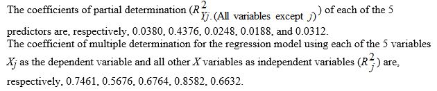
TABLE 14-15 The superintendent of a school district wanted to predict the percentage of students passing a sixth-grade proficiency test. She obtained the data on percentage of students passing the proficiency test (% Passing), daily mean of the percentage of students attending class (% Attendance), mean teacher salary in dollars (Salaries), and instructional spending per pupil in dollars (Spending) of 47 schools in the state. Following is the multiple regression output with Y = % Passing as the dependent variable, X₁ = % Attendance, X₂= Salaries and X₃= Spending: 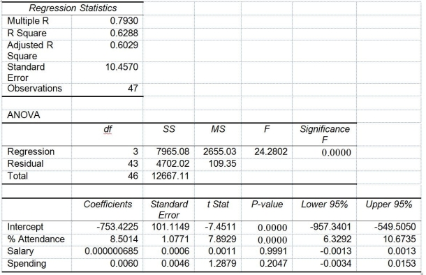-Referring to Table 14-15, the alternative hypothesis H₁: At least one of βⱼ ≠ 0 for j = 1, 2, 3 implies that percentage of students passing the proficiency test is affected by all of the explanatory variables.

TABLE 14-19 The marketing manager for a nationally franchised lawn service company would like to study the characteristics that differentiate home owners who do and do not have a lawn service. A random sample of 30 home owners located in a suburban area near a large city was selected; 15 did not have a lawn service (code 0) and 15 had a lawn service (code 1). Additional information available concerning these 30 home owners includes family income (Income, in thousands of dollars), lawn size (Lawn Size, in thousands of square feet), attitude toward outdoor recreational activities (Atitude 0 = unfavorable, 1 = favorable), number of teenagers in the household (Teenager), and age of the head of the household (Age). The Minitab output is given below: 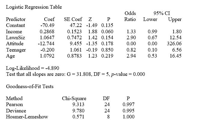-Referring to Table 14-19, what is the p-value of the test statistic when testing whether Income makes a significant contribution to the model in the presence of the other independent variables?

TABLE 14-8 A financial analyst wanted to examine the relationship between salary (in $1,000) and 4 variables: age (X₁ = Age), experience in the field (X₂ = Exper), number of degrees (X₃ = Degrees), and number of previous jobs in the field (X₄ = Prevjobs). He took a sample of 20 employees and obtained the following Microsoft Excel output: 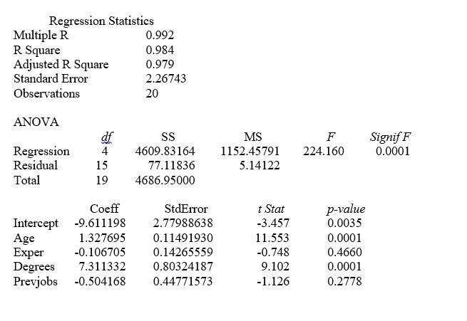-Referring to Table 14-8, the analyst wants to use a t test to test for the significance of the coefficient of X₃. The value of the test statistic is ________.

TABLE 14-11 A weight-loss clinic wants to use regression analysis to build a model for weight-loss of a client (measured in pounds). Two variables thought to affect weight-loss are client's length of time on the weight-loss program and time of session. These variables are described below: Y = Weight-loss (in pounds) X₁ = Length of time in weight-loss program (in months) X₂ = 1 if morning session, 0 if not X₃ = 1 if afternoon session, 0 if not (Base level = evening session) Data for 12 clients on a weight-loss program at the clinic were collected and used to fit the interaction model: Y = β₀ + β₁X₁ + β₂X₂ + β₃X₃ + β₄X₁X₂ + β₅X₁X₂ + ε Partial output from Microsoft Excel follows: 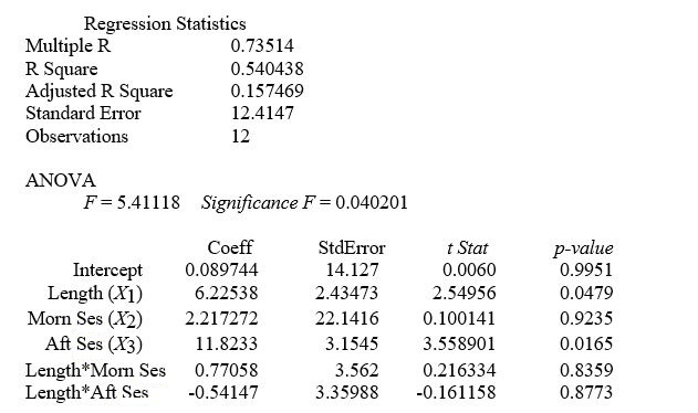-Referring to Table 14-11, in terms of the βs in the model, give the mean change in weight-loss (Y) for every 1 month increase in time in the program (X₁) when attending the evening session.

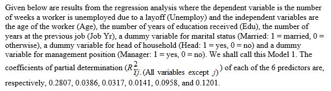
TABLE 14-17 Model 2 is the regression analysis where the dependent variable is Unemploy and the independent variables are Age and Manager. The results of the regression analysis are given below: -Referring to Table 14-17 Model 1, ________ of the variation in the number of weeks a worker is unemployed due to a layoff can be explained by the number of years at the previous job while controlling for the other independent variables.

TABLE 14-15 The superintendent of a school district wanted to predict the percentage of students passing a sixth-grade proficiency test. She obtained the data on percentage of students passing the proficiency test (% Passing), daily mean of the percentage of students attending class (% Attendance), mean teacher salary in dollars (Salaries), and instructional spending per pupil in dollars (Spending) of 47 schools in the state. Following is the multiple regression output with Y = % Passing as the dependent variable, X₁ = % Attendance, X₂= Salaries and X₃= Spending: -Referring to Table 14-15, what are the lower and upper limits of the 95% confidence interval estimate for the effect of a one dollar increase in mean teacher salary on the mean percentage of students passing the proficiency test?

TABLE 14-19 The marketing manager for a nationally franchised lawn service company would like to study the characteristics that differentiate home owners who do and do not have a lawn service. A random sample of 30 home owners located in a suburban area near a large city was selected; 15 did not have a lawn service (code 0) and 15 had a lawn service (code 1). Additional information available concerning these 30 home owners includes family income (Income, in thousands of dollars), lawn size (Lawn Size, in thousands of square feet), attitude toward outdoor recreational activities (Atitude 0 = unfavorable, 1 = favorable), number of teenagers in the household (Teenager), and age of the head of the household (Age). The Minitab output is given below: -Referring to Table 14-19, there is not enough evidence to conclude that the model is not a good-fitting model at a 0.05 level of significance.

TABLE 14-6 One of the most common questions of prospective house buyers pertains to the cost of heating in dollars (Y). To provide its customers with information on that matter, a large real estate firm used the following 4 variables to predict heating costs: the daily minimum outside temperature in degrees of Fahrenheit (X₁) the amount of insulation in inches (X₂), the number of windows in the house (X₃), and the age of the furnace in years (X₄). Given below are the Excel outputs of two regression models. Model 1 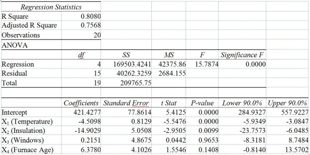Model 2 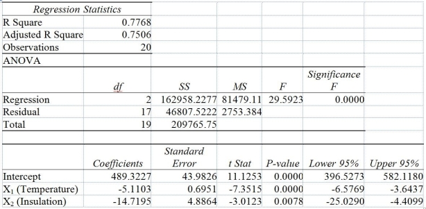-Referring to Table 14-6, what is the value of the partial F test statistic for H₀: β₃ = β₄ = 0 vs. H₁: At least one βⱼ ≠ 0, j = 3, 4?

TABLE 14-10 You worked as an intern at We Always Win Car Insurance Company last summer. You notice that individual car insurance premiums depend very much on the age of the individual, the number of traffic tickets received by the individual, and the population density of the city in which the individual lives. You performed a regression analysis in Excel and obtained the following information: 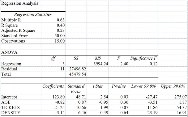-Referring to Table 14-10, the 99% confidence interval for the change in mean insurance premiums of a person who has become 1 year older (i.e., the slope coefficient for AGE) is ?-0.82 ± ________.

TABLE 14-19 The marketing manager for a nationally franchised lawn service company would like to study the characteristics that differentiate home owners who do and do not have a lawn service. A random sample of 30 home owners located in a suburban area near a large city was selected; 15 did not have a lawn service (code 0) and 15 had a lawn service (code 1). Additional information available concerning these 30 home owners includes family income (Income, in thousands of dollars), lawn size (Lawn Size, in thousands of square feet), attitude toward outdoor recreational activities (Atitude 0 = unfavorable, 1 = favorable), number of teenagers in the household (Teenager), and age of the head of the household (Age). The Minitab output is given below: -Referring to Table 14-19, which of the following is the correct interpretation for the Income slope coefficient?

TABLE 14-13 An econometrician is interested in evaluating the relationship of demand for building materials to mortgage rates in Los Angeles and San Francisco. He believes that the appropriate model is Y = 10 + 5X₁ + 8X₂ where X₁ = mortgage rate in % X₂ = 1 if SF, 0 if LA Y = demand in $100 per capita -Referring to Table 14-13, holding constant the effect of city, each additional increase of 1% in the mortgage rate would lead to an estimated increase of ________ in the mean demand.

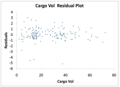
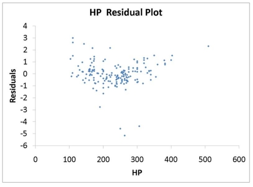
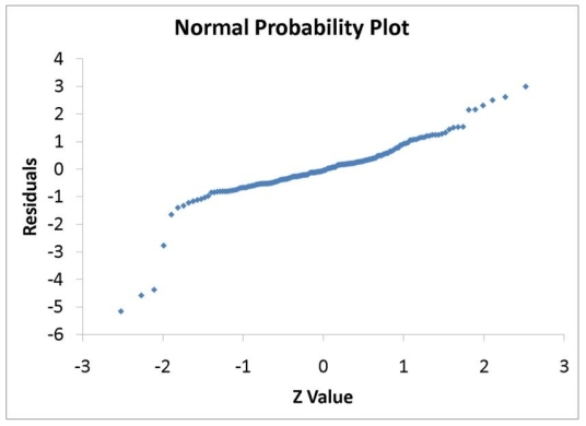
TABLE 14-16 What are the factors that determine the acceleration time (in sec.) from 0 to 60 miles per hour of a car? Data on the following variables for 171 different vehicle models were collected: Accel Time: Acceleration time in sec. Cargo Vol: Cargo volume in cu. ft. HP: Horsepower MPG: Miles per gallon SUV: 1 if the vehicle model is an SUV with Coupe as the base when SUV and Sedan are both 0 Sedan: 1 if the vehicle model is a sedan with Coupe as the base when SUV and Sedan are both 0 The regression results using acceleration time as the dependent variable and the remaining variables as the independent variables are presented below. 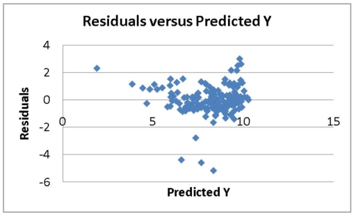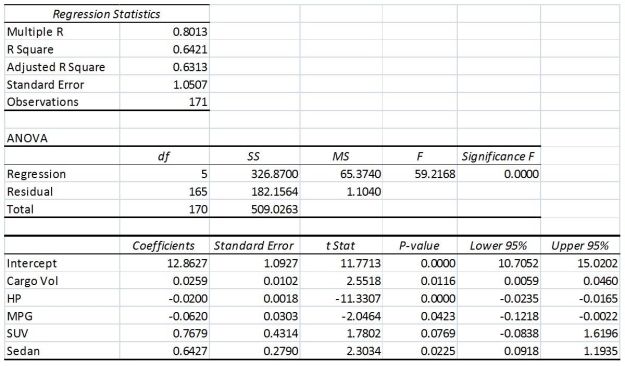The various residual plots are as shown below. -Referring to 14-16, the 0 to 60 miles per hour acceleration time of a coupe is predicted to be 0.7679 seconds lower than that of an SUV.

TABLE 14-6 One of the most common questions of prospective house buyers pertains to the cost of heating in dollars (Y). To provide its customers with information on that matter, a large real estate firm used the following 4 variables to predict heating costs: the daily minimum outside temperature in degrees of Fahrenheit (X₁) the amount of insulation in inches (X₂), the number of windows in the house (X₃), and the age of the furnace in years (X₄). Given below are the Excel outputs of two regression models. Model 1 Model 2 -Referring to Table 14-6, what is the 90% confidence interval for the expected change in heating costs as a result of a 1 degree Fahrenheit change in the daily minimum outside temperature using Model 1?

TABLE 14-10 You worked as an intern at We Always Win Car Insurance Company last summer. You notice that individual car insurance premiums depend very much on the age of the individual, the number of traffic tickets received by the individual, and the population density of the city in which the individual lives. You performed a regression analysis in Excel and obtained the following information: -Referring to Table 14-10, the total degrees of freedom that are missing in the ANOVA table should be ________.

TABLE 14-16 What are the factors that determine the acceleration time (in sec.) from 0 to 60 miles per hour of a car? Data on the following variables for 171 different vehicle models were collected: Accel Time: Acceleration time in sec. Cargo Vol: Cargo volume in cu. ft. HP: Horsepower MPG: Miles per gallon SUV: 1 if the vehicle model is an SUV with Coupe as the base when SUV and Sedan are both 0 Sedan: 1 if the vehicle model is a sedan with Coupe as the base when SUV and Sedan are both 0 The regression results using acceleration time as the dependent variable and the remaining variables as the independent variables are presented below. The various residual plots are as shown below. -Referring to 14-16, what is the value of the test statistic to determine whether Cargo Vol makes a significant contribution to the regression model in the presence of the other independent variables at a 5% level of significance?

TABLE 14-18 A logistic regression model was estimated in order to predict the probability that a randomly chosen university or college would be a private university using information on mean total Scholastic Aptitude Test score (SAT) at the university or college, the room and board expense measured in thousands of dollars (Room/Brd), and whether the TOEFL criterion is at least 550 (Toefl550 = 1 if yes, 0 otherwise.) The dependent variable, Y, is school type (Type = 1 if private and 0 otherwise). The Minitab output is given below: 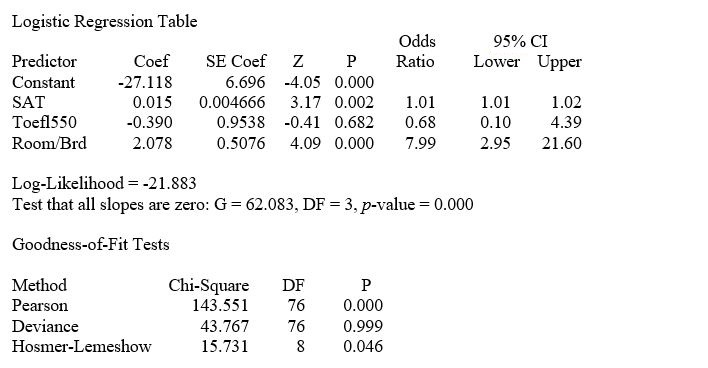-Referring to Table 14-18, what should be the decision ('reject' or 'do not reject') on the null hypothesis when testing whether Toefl500 makes a significant contribution to the model in the presence of the other independent variables at a 0.05 level of significance?

TABLE 14-2 A professor of industrial relations believes that an individual's wage rate at a factory (Y) depends on his performance rating (X₁) and the number of economics courses the employee successfully completed in college (X₂). The professor randomly selects 6 workers and collects the following information: 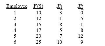-Referring to Table 14-2, an employee who took 12 economics courses scores 10 on the performance rating. What is her estimated expected wage rate?

The coefficient of multiple determination measures the proportion of the total variation in the dependent variable that is explained by the set of independent variables.

TABLE 14-12 As a project for his business statistics class, a student examined the factors that determined parking meter rates throughout the campus area. Data were collected for the price per hour of parking, blocks to the quadrangle, and one of the three jurisdictions: on campus, in downtown and off campus, or outside of downtown and off campus. The population regression model hypothesized is Yᵢ = α + β₁X₁ᵢ + β₂X₂ᵢ + β₃X₃ᵢ + ε where Y is the meter price X₁ is the number of blocks to the quad X₂ is a dummy variable that takes the value 1 if the meter is located in downtown and off campus and the value 0 otherwise X₃ is a dummy variable that takes the value 1 if the meter is located outside of downtown and off campus, and the value 0 otherwise The following Excel results are obtained. 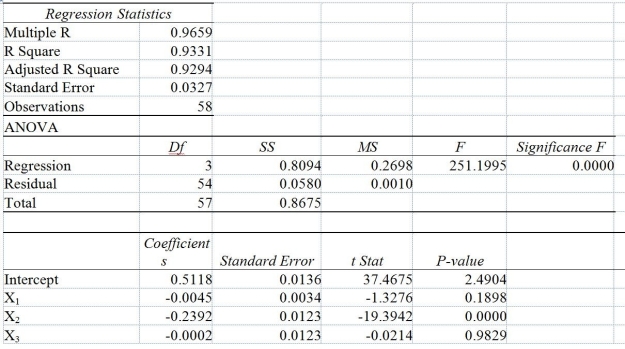-Referring to Table 14-12, if one is already outside of downtown and off campus but decides to park 3 more blocks from the quad, the estimated mean parking meter rate will

TABLE 14-16 What are the factors that determine the acceleration time (in sec.) from 0 to 60 miles per hour of a car? Data on the following variables for 171 different vehicle models were collected: Accel Time: Acceleration time in sec. Cargo Vol: Cargo volume in cu. ft. HP: Horsepower MPG: Miles per gallon SUV: 1 if the vehicle model is an SUV with Coupe as the base when SUV and Sedan are both 0 Sedan: 1 if the vehicle model is a sedan with Coupe as the base when SUV and Sedan are both 0 The regression results using acceleration time as the dependent variable and the remaining variables as the independent variables are presented below. The various residual plots are as shown below. -Referring to 14-16, what is the value of the test statistic to determine whether HP makes a significant contribution to the regression model in the presence of the other independent variables at a 5% level of significance?