Exam 14: Introduction to Multiple Regression

TABLE 14-15 The superintendent of a school district wanted to predict the percentage of students passing a sixth-grade proficiency test. She obtained the data on percentage of students passing the proficiency test (% Passing), daily mean of the percentage of students attending class (% Attendance), mean teacher salary in dollars (Salaries), and instructional spending per pupil in dollars (Spending) of 47 schools in the state. Following is the multiple regression output with Y = % Passing as the dependent variable, X₁ = % Attendance, X₂= Salaries and X₃= Spending: Regression Statistics Multiple R 0.7930 R Square 0.6288 Adjusted R 0.6029 Square Standard 10.4570 Error Observations 47 $\text { ANOVA }$ df SS MS Significance F Regression 3 7965.08 2655.03 24.2802 0.0000 Residual 43 4702.02 109.35 Total 46 12667.11 Coefficients Standard Error t Stat P-value Lower 95\% Upper 95\% Intercept -753.4225 101.1149 -7.4511 0.0000 -957.3401 -549.5050 \% Attendance 8.5014 1.0771 7.8929 0.0000 6.3292 10.6735 Salary 0.000000685 0.0006 0.0011 0.9991 -0.0013 0.0013 Spending 0.0060 0.0046 1.2879 0.2047 -0.0034 0.0153 -Referring to Table 14-15, the alternative hypothesis H?: At least one of ?? ? 0 for j = 1, 2, 3 implies that percentage of students passing the proficiency test is affected by all of the explanatory variables.

TABLE 14-5 A microeconomist wants to determine how corporate sales are influenced by capital and wage spending by companies. She proceeds to randomly select 26 large corporations and record information in millions of dollars. The Microsoft Excel output below shows results of this multiple regression. SUMMARY OUTPUT Regression Statistics Multiple R 0.830 R Square 0.689 Adjusted R Square 0.662 Standard Error 17501.643 Observations 26 ANOVA df SS MS F Signif F Regression 2 15579777040 7789888520 25.432 0.0001 Residual 23 7045072780 306307512 Total 25 22624849820 Coeff StdError t Stat p -value Intercept 15800.0000 6038.2999 2.617 0.0154 Capital 0.1245 0.2045 0.609 0.5485 Wages 7.0762 1.4729 4.804 0.0001 -Referring to Table 14-5, which of the independent variables in the model are significant at the 5% level?

TABLE 14-17 Given below are results from the regression analysis where the dependent variable is the number of weeks a worker is unemployed due to a layoff (Unemploy) and the independent variables are the age of the worker (Age), the number of years of education received (Edu), the number of years at the previous job (Job Yr), a dummy variable for marital status (Married: 1 = married, 0 = otherwise), a dummy variable for head of household (Head: 1 = yes, 0 = no) and a dummy variable for management position (Manager: 1 = yes, 0 = no). We shall call this Model 1. The coefficients of partial determination ( 2 Yj. (Allvariables except $j$ ) ) of each of the 6 predictors are, respectively, 0.2807, 0.0386, 0.0317, 0.0141, 0.0958, and 0.1201. Regression Statistics Multiple R 0.7035 R Square 0.4949 Adjusted R 0.4030 Square Standard 18.4861 Error 40 Observations $\text { ANOVA }$ df SS MS F significance F Regression 6 11048.6415 1841.4402 5.3885 0.00057 Residual 33 11277.2586 341.7351 Total 39 22325.9 Coefficients Standard Error t Stat P-value Lower 95\% Upper 95\% Intercept 32.6595 23.18302 1.4088 0.1683 -14.5067 79.8257 Age 1.2915 0.3599 3.5883 0.0011 0.5592 2.0238 Edu -1.3537 1.1766 -1.1504 0.2582 -3.7476 1.0402 Job Yr 0.6171 0.5940 1.0389 0.3064 -0.5914 1.8257 Married -5.2189 7.6068 -0.6861 0.4974 -20.6950 10.2571 Head -14.2978 7.6479 -1.8695 0.0704 -29.8575 1.2618 Manager -24.8203 11.6932 -2.1226 0.0414 -48.6102 -1.0303 Model 2 is the regression analysis where the dependent variable is Unemploy and the independent variables are Age and Manager. The results of the regression analysis are given below: Regression Statistics Multiple R 0.6391 R Square 0.4085 Adjusted R 0.3765 Square Standard Error 18.8929 Observations 40 $\text { ANOVA }$ df SS MS F Significance F Regression 2 9119.0897 4559.5448 12.7740 0.0000 Residual 37 13206.8103 356.9408 Total 39 22325.9 Coefficients Standard Error t Stat P -value Intercept -0.2143 11.5796 -0.0185 0.9853 Age 1.4448 0.3160 4.5717 0.0000 Manager -22.5761 11.3488 -1.9893 0.0541 -Referring to Table 14-17 Model 1, what are the lower and upper limits of the 95% confidence interval estimate for the difference in the mean number of weeks a worker is unemployed due to a layoff between a worker who is married and one who is not after taking into consideration the effect of all the other independent variables?

TABLE 14-15 The superintendent of a school district wanted to predict the percentage of students passing a sixth-grade proficiency test. She obtained the data on percentage of students passing the proficiency test (% Passing), daily mean of the percentage of students attending class (% Attendance), mean teacher salary in dollars (Salaries), and instructional spending per pupil in dollars (Spending) of 47 schools in the state. Following is the multiple regression output with Y = % Passing as the dependent variable, X₁ = % Attendance, X₂= Salaries and X₃= Spending: Regression Statistics Multiple R 0.7930 R Square 0.6288 Adjusted R 0.6029 Square Standard 10.4570 Error Observations 47 $\text { ANOVA }$ df SS MS Significance F Regression 3 7965.08 2655.03 24.2802 0.0000 Residual 43 4702.02 109.35 Total 46 12667.11 Coefficients Standard Error t Stat P-value Lower 95\% Upper 95\% Intercept -753.4225 101.1149 -7.4511 0.0000 -957.3401 -549.5050 \% Attendance 8.5014 1.0771 7.8929 0.0000 6.3292 10.6735 Salary 0.000000685 0.0006 0.0011 0.9991 -0.0013 0.0013 Spending 0.0060 0.0046 1.2879 0.2047 -0.0034 0.0153 -Referring to Table 14-15, estimate the mean percentage of students passing the proficiency test for all the schools that have a daily mean of 95% of students attending class, an mean teacher salary of 40,000 dollars, and an instructional spending per pupil of 2,000 dollars.

TABLE 14-1 A manager of a product sales group believes the number of sales made by an employee (Y) depends on how many years that employee has been with the company (X₁) and how he/she scored on a business aptitude test (X₂). A random sample of 8 employees provides the following: 1 100 10 7 2 90 3 10 3 80 8 9 4 70 5 4 5 60 5 8 6 50 7 5 7 40 1 4 8 30 1 1 -Referring to Table 14-1, if an employee who had been with the company 5 years scored a 9 on the aptitude test, what would his estimated expected sales be?

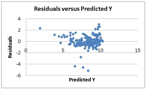
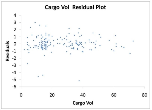
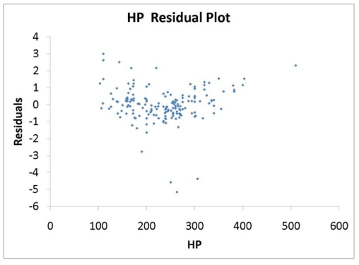
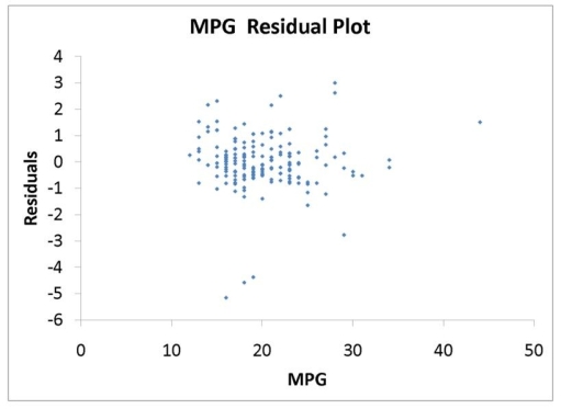
TABLE 14-16 What are the factors that determine the acceleration time (in sec.) from 0 to 60 miles per hour of a car? Data on the following variables for 171 different vehicle models were collected: Accel Time: Acceleration time in sec. Cargo Vol: Cargo volume in cu. ft. HP: Horsepower MPG: Miles per gallon SUV: 1 if the vehicle model is an SUV with Coupe as the base when SUV and Sedan are both 0 Sedan: 1 if the vehicle model is a sedan with Coupe as the base when SUV and Sedan are both 0 The regression results using acceleration time as the dependent variable and the remaining variables as the independent variables are presented below. Regression Statistics Multiple R 0.8013 R Square 0.6421 Adjusted R Square 0.6313 Standard Error 1.0507 Observations 171 $\text { ANOVA }$ df SS MS F Significance F Regression 5 326.8700 65.3740 59.2168 0.0000 Residual 165 182.1564 1.1040 Total 170 509.0263 Coefficients Standard Error t Stat P-value Lower 95\% Upper 95\% Intercept 12.8627 1.0927 11.7713 0.0000 10.7052 15.0202 Cargo Vol 0.0259 0.0102 2.5518 0.0116 0.0059 0.0460 HP -0.0200 0.0018 -11.3307 0.0000 -0.0235 -0.0165 MPG -0.0620 0.0303 -2.0464 0.0423 -0.1218 -0.0022 SUV 0.7679 0.4314 1.7802 0.0769 -0.0838 1.6196 Sedan 0.6427 0.2790 2.3034 0.0225 0.0918 1.1935 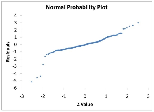The various residual plots are as shown below. The coefficients of partial determination $\left( R ^ { 2 }_{Y j} \right.$ . (All variables except $\left. j \right)$ of each of the 5 predictors are, respectively, $0.0380,0.4376,0.0248,0.0188$ , and $0.0312$ . The coefficient of multiple determination for the regression model using each of the 5 variables $X _ { j }$ as the dependent variable and all other $X$ variables as independent variables $\left( R _ { j } ^ { 2 } \right)$ are, respectively, $0.7461,0.5676,0.6764,0.8582,0.6632$ . -Referring to 14-16, there is enough evidence to conclude that SUV makes a significant contribution to the regression model in the presence of the other independent variables at a 5% level of significance.

TABLE 14-17 Given below are results from the regression analysis where the dependent variable is the number of weeks a worker is unemployed due to a layoff (Unemploy) and the independent variables are the age of the worker (Age), the number of years of education received (Edu), the number of years at the previous job (Job Yr), a dummy variable for marital status (Married: 1 = married, 0 = otherwise), a dummy variable for head of household (Head: 1 = yes, 0 = no) and a dummy variable for management position (Manager: 1 = yes, 0 = no). We shall call this Model 1. The coefficients of partial determination ( 2 Yj. (Allvariables except $j$ ) ) of each of the 6 predictors are, respectively, 0.2807, 0.0386, 0.0317, 0.0141, 0.0958, and 0.1201. Regression Statistics Multiple R 0.7035 R Square 0.4949 Adjusted R 0.4030 Square Standard 18.4861 Error 40 Observations $\text { ANOVA }$ df SS MS F significance F Regression 6 11048.6415 1841.4402 5.3885 0.00057 Residual 33 11277.2586 341.7351 Total 39 22325.9 Coefficients Standard Error t Stat P-value Lower 95\% Upper 95\% Intercept 32.6595 23.18302 1.4088 0.1683 -14.5067 79.8257 Age 1.2915 0.3599 3.5883 0.0011 0.5592 2.0238 Edu -1.3537 1.1766 -1.1504 0.2582 -3.7476 1.0402 Job Yr 0.6171 0.5940 1.0389 0.3064 -0.5914 1.8257 Married -5.2189 7.6068 -0.6861 0.4974 -20.6950 10.2571 Head -14.2978 7.6479 -1.8695 0.0704 -29.8575 1.2618 Manager -24.8203 11.6932 -2.1226 0.0414 -48.6102 -1.0303 Model 2 is the regression analysis where the dependent variable is Unemploy and the independent variables are Age and Manager. The results of the regression analysis are given below: Regression Statistics Multiple R 0.6391 R Square 0.4085 Adjusted R 0.3765 Square Standard Error 18.8929 Observations 40 $\text { ANOVA }$ df SS MS F Significance F Regression 2 9119.0897 4559.5448 12.7740 0.0000 Residual 37 13206.8103 356.9408 Total 39 22325.9 Coefficients Standard Error t Stat P -value Intercept -0.2143 11.5796 -0.0185 0.9853 Age 1.4448 0.3160 4.5717 0.0000 Manager -22.5761 11.3488 -1.9893 0.0541 -Referring to Table 14-17 and using both Model 1 and Model 2, there is sufficient evidence to conclude that the independent variables that are not significant individually are also not significant as a group in explaining the variation in the dependent variable at a 5% level of significance?

TABLE 14-12 As a project for his business statistics class, a student examined the factors that determined parking meter rates throughout the campus area. Data were collected for the price per hour of parking, blocks to the quadrangle, and one of the three jurisdictions: on campus, in downtown and off campus, or outside of downtown and off campus. The population regression model hypothesized is Yᵢ = α + β₁X₁ᵢ + β₂X₂ᵢ + β₃X₃ᵢ + ε where Y is the meter price X₁ is the number of blocks to the quad X₂ is a dummy variable that takes the value 1 if the meter is located in downtown and off campus and the value 0 otherwise X₃ is a dummy variable that takes the value 1 if the meter is located outside of downtown and off campus, and the value 0 otherwise The following Excel results are obtained. Regression Statistics Multiple R 0.9659 R Square 0.9331 Adjusted R Square 0.9294 Standard Error 0.0327 Observations 58 $\text { ANOVA }$ Df SS MS F Significance F Regression 3 0.8094 0.2698 251.1995 0.0000 Residual 54 0.0580 0.0010 Total 57 0.8675 Coefficient Standard Error S Stat P-value Intercept 0.5118 0.0136 37.4675 2.4904 -0.0045 0.0034 -1.3276 0.1898 -0.2392 0.0123 -19.3942 0.0000 -0.0002 0.0123 -0.0214 0.9829 -Referring to Table 14-12, if one is already outside of downtown and off campus but decides to park 3 more blocks from the quad, the estimated mean parking meter rate will

TABLE 14-7 The department head of the accounting department wanted to see if she could predict the GPA of students using the number of course units (credits) and total SAT scores of each. She takes a sample of students and generates the following Microsoft Excel output: SUMMARY OUTPUT SUMMARY OUTPUT Regression Statistics Multiple R 0.916 R Square 0.839 Adjusted R Square 0.732 Standard Error 0.24685 Observations 6 ANOVA df SS MS F Signif F Regression 2 0.95219 0.47610 7.813 0.0646 Residual 3 0.18281 0.06094 Total 5 1.13500 Coeff StdError t Stat p -value Intercept 4.593897 1.13374542 4.052 0.0271 Units -0.247270 0.06268485 -3.945 0.0290 SAT Total 0.001443 0.00101241 1.425 0.2494 -Referring to Table 14-7, the value of the coefficient of multiple determination, r²Y.₁₂, is ________.

TABLE 14-15 The superintendent of a school district wanted to predict the percentage of students passing a sixth-grade proficiency test. She obtained the data on percentage of students passing the proficiency test (% Passing), daily mean of the percentage of students attending class (% Attendance), mean teacher salary in dollars (Salaries), and instructional spending per pupil in dollars (Spending) of 47 schools in the state. Following is the multiple regression output with Y = % Passing as the dependent variable, X₁ = % Attendance, X₂= Salaries and X₃= Spending: Regression Statistics Multiple R 0.7930 R Square 0.6288 Adjusted R 0.6029 Square Standard 10.4570 Error Observations 47 $\text { ANOVA }$ df SS MS Significance F Regression 3 7965.08 2655.03 24.2802 0.0000 Residual 43 4702.02 109.35 Total 46 12667.11 Coefficients Standard Error t Stat P-value Lower 95\% Upper 95\% Intercept -753.4225 101.1149 -7.4511 0.0000 -957.3401 -549.5050 \% Attendance 8.5014 1.0771 7.8929 0.0000 6.3292 10.6735 Salary 0.000000685 0.0006 0.0011 0.9991 -0.0013 0.0013 Spending 0.0060 0.0046 1.2879 0.2047 -0.0034 0.0153 -Referring to Table 14-15, which of the following is a correct statement?

In a multiple regression problem involving two independent variables, if b₁ is computed to be +2.0, it means that

TABLE 14-8 A financial analyst wanted to examine the relationship between salary (in $1,000) and 4 variables: age (X₁ = Age), experience in the field (X₂ = Exper), number of degrees (X₃ = Degrees), and number of previous jobs in the field (X₄ = Prevjobs). He took a sample of 20 employees and obtained the following Microsoft Excel output: SUMMARY OUTPUT Regression Statistics Multiple R 0.992 R Square 0.984 Adjusted R Square 0.979 Standard Error 2.26743 Observations 20 ANOVA df SS MS F Signif F Regression 4 4609.83164 1152.45791 224.160 0.0001 Residual 15 77.11836 5.14122 Total 19 4686.95000 Coeff StdError t Stat p -value Intercept -9.611198 2.77988638 -3.457 0.0035 Age 1.327695 0.11491930 11.553 0.0001 Exper -0.106705 0.14265559 -0.748 0.4660 Degrees 7.311332 0.80324187 9.102 0.0001 Prevjobs -0.504168 0.44771573 -1.126 0.2778 -Referring to Table 14-8, the value of the coefficient of multiple determination, r²Y.₁₂₃₄, is ________.

An interaction term in a multiple regression model may be used when

TABLE 14-5 A microeconomist wants to determine how corporate sales are influenced by capital and wage spending by companies. She proceeds to randomly select 26 large corporations and record information in millions of dollars. The Microsoft Excel output below shows results of this multiple regression. SUMMARY OUTPUT Regression Statistics Multiple R 0.830 R Square 0.689 Adjusted R Square 0.662 Standard Error 17501.643 Observations 26 ANOVA df SS MS F Signif F Regression 2 15579777040 7789888520 25.432 0.0001 Residual 23 7045072780 306307512 Total 25 22624849820 Coeff StdError t Stat p -value Intercept 15800.0000 6038.2999 2.617 0.0154 Capital 0.1245 0.2045 0.609 0.5485 Wages 7.0762 1.4729 4.804 0.0001 -Referring to Table 14-5, what is the p-value for Wages?

TABLE 14-10 You worked as an intern at We Always Win Car Insurance Company last summer. You notice that individual car insurance premiums depend very much on the age of the individual, the number of traffic tickets received by the individual, and the population density of the city in which the individual lives. You performed a regression analysis in Excel and obtained the following information: $\text { Regression Analysis }$ Regression Statistics Multiple R 0.63 R Square 0.40 Adjusted R Square 0.23 Standard Error 50.00 Observations 15.00 $\text { ANOVA }$ df SS MS F Significance F Regression 3 5994.24 2.40 0.12 Residual 11 27496.82 Total 45479.54 Coefficients Standard Error t Stat P-value Lower 99.0\% Upper 99.0\% Intercept 123.80 48.71 2.54 0.03 -27.47 275.07 AGE -0.82 0.87 -0.95 0.36 -3.51 1.87 TICKETS 21.25 10.66 1.99 0.07 -11.86 54.37 DENSITY -3.14 6.46 -0.49 0.64 -23.19 16.91 -Referring to Table 14-10, to test the significance of the multiple regression model, what are the degrees of freedom?