Exam 13: Introduction to Multiple Regression

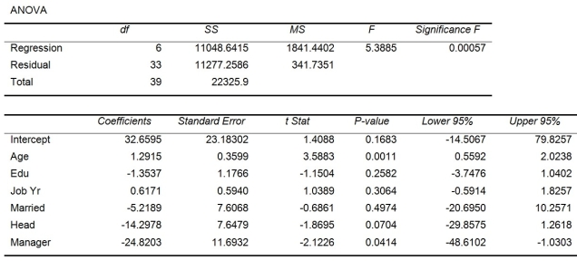
TABLE 13-17 Given below are results from the regression analysis where the dependent variable is the number of weeks a worker is unemployed due to a layoff (Unemploy) and the independent variables are the age of the worker (Age), the number of years of education received (Edu), the number of years at the previous job (Job Yr), a dummy variable for marital status (Married: 1 = married, 0 = otherwise), a dummy variable for head of household (Head: 1 = yes, 0 = no) and a dummy variable for management position (Manager: 1 = yes, 0 = no). We shall call this Model 1. 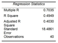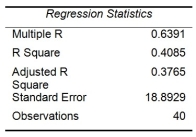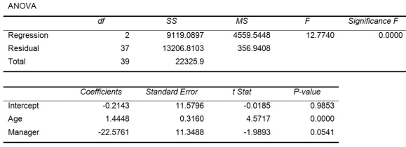Model 2 is the regression analysis where the dependent variable is Unemploy and the independent variables are Age and Manager. The results of the regression analysis are given below: -Referring to Table 13-17 Model 1, the alternative hypothesis H₁: At least one of βⱼ ≠ 0 for j = 1, 2, 3, 4, 5, 6 implies that the number of weeks a worker is unemployed due to a layoff is affected by at least one of the explanatory variables.

TABLE 13-17 Given below are results from the regression analysis where the dependent variable is the number of weeks a worker is unemployed due to a layoff (Unemploy) and the independent variables are the age of the worker (Age), the number of years of education received (Edu), the number of years at the previous job (Job Yr), a dummy variable for marital status (Married: 1 = married, 0 = otherwise), a dummy variable for head of household (Head: 1 = yes, 0 = no) and a dummy variable for management position (Manager: 1 = yes, 0 = no). We shall call this Model 1. Model 2 is the regression analysis where the dependent variable is Unemploy and the independent variables are Age and Manager. The results of the regression analysis are given below: -Referring to Table 13-17 Model 1, what are the lower and upper limits of the 95% confidence interval estimate for the effect of a one year increase in education received on the mean number of weeks a worker is unemployed due to a layoff after taking into consideration the effect of all the other independent variables?

TABLE 13-12 As a project for his business statistics class, a student examined the factors that determined parking meter rates throughout the campus area. Data were collected for the price per hour of parking, blocks to the quadrangle, and one of the three jurisdictions: on campus, in downtown and off campus, or outside of downtown and off campus. The population regression model hypothesized is Yi = α + β1X1i + β2X2i + β3X3i + ε where Y is the meter price X1 is the number of blocks to the quad X2 is a dummy variable that takes the value 1 if the meter is located in downtown and off campus and the value 0 otherwise X3 is a dummy variable that takes the value 1 if the meter is located outside of downtown and off campus, and the value 0 otherwise The following Microsoft Excel results are obtained. -In trying to construct a model to estimate grades on a statistics test, a professor wanted to include, among other factors, whether the person had taken the course previously. To do this, the professor included a dummy variable in her regression model that was equal to 1 if the person had previously taken the course, and 0 otherwise. The interpretation of the coefficient associated with this dummy variable would be the mean amount the repeat students tended to be above or below non-repeaters, with all other factors the same.

TABLE 13-5 A microeconomist wants to determine how corporate sales are influenced by capital and wage spending by companies. She proceeds to randomly select 26 large corporations and record information in millions of dollars. The Microsoft Excel output below shows results of this multiple regression. 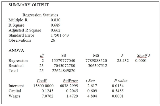-Referring to Table 13-5, the observed value of the F-statistic is given on the printout as 25.432. What are the degrees of freedom for this F-statistic?

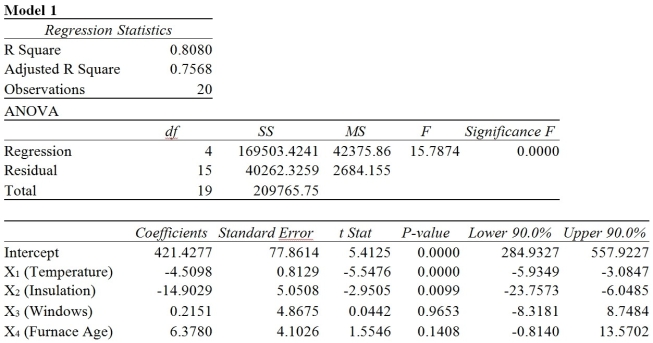
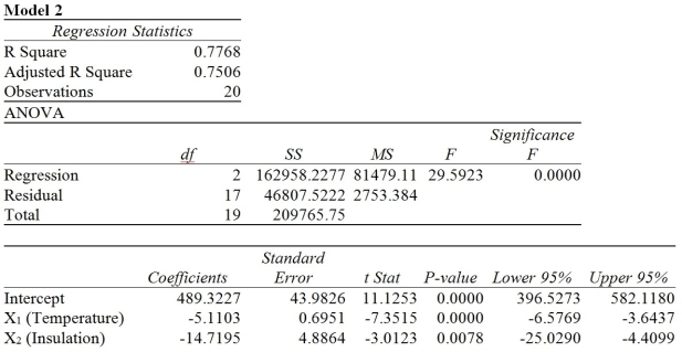
TABLE 13-6 One of the most common questions of prospective house buyers pertains to the cost of heating in dollars (Y). To provide its customers with information on that matter, a large real estate firm used the following four variables to predict heating costs: the daily minimum outside temperature in degrees of Fahrenheit (X1), the amount of insulation in inches (X2), the number of windows in the house (X3), and the age of the furnace in years (X4). Given below are the Microsoft Excel outputs of two regression models. -The total sum of squares (SST)in a regression model will never be greater than the regression sum of squares (SSR).

TABLE 13-17 Given below are results from the regression analysis where the dependent variable is the number of weeks a worker is unemployed due to a layoff (Unemploy) and the independent variables are the age of the worker (Age), the number of years of education received (Edu), the number of years at the previous job (Job Yr), a dummy variable for marital status (Married: 1 = married, 0 = otherwise), a dummy variable for head of household (Head: 1 = yes, 0 = no) and a dummy variable for management position (Manager: 1 = yes, 0 = no). We shall call this Model 1. Model 2 is the regression analysis where the dependent variable is Unemploy and the independent variables are Age and Manager. The results of the regression analysis are given below: -Referring to Table 13-17 Model 1, which of the following is a correct statement?

TABLE 13-5 A microeconomist wants to determine how corporate sales are influenced by capital and wage spending by companies. She proceeds to randomly select 26 large corporations and record information in millions of dollars. The Microsoft Excel output below shows results of this multiple regression. -Referring to Table 13-5, one company in the sample had sales of $21.439 billion (Sales = 21,439). This company spent $300 million on capital and $700 million on wages. What is the residual (in millions of dollars)for this data point?

TABLE 13-6 One of the most common questions of prospective house buyers pertains to the cost of heating in dollars (Y). To provide its customers with information on that matter, a large real estate firm used the following four variables to predict heating costs: the daily minimum outside temperature in degrees of Fahrenheit (X1), the amount of insulation in inches (X2), the number of windows in the house (X3), and the age of the furnace in years (X4). Given below are the Microsoft Excel outputs of two regression models. -The coefficient of multiple determination, r², measures the proportion of variation in Y that is explained by X₁ and X₂.

TABLE 13-5 A microeconomist wants to determine how corporate sales are influenced by capital and wage spending by companies. She proceeds to randomly select 26 large corporations and record information in millions of dollars. The Microsoft Excel output below shows results of this multiple regression. -Referring to Table 13-5, which of the following values for α is the smallest for which the regression model as a whole is significant?

TABLE 13-17 Given below are results from the regression analysis where the dependent variable is the number of weeks a worker is unemployed due to a layoff (Unemploy) and the independent variables are the age of the worker (Age), the number of years of education received (Edu), the number of years at the previous job (Job Yr), a dummy variable for marital status (Married: 1 = married, 0 = otherwise), a dummy variable for head of household (Head: 1 = yes, 0 = no) and a dummy variable for management position (Manager: 1 = yes, 0 = no). We shall call this Model 1. Model 2 is the regression analysis where the dependent variable is Unemploy and the independent variables are Age and Manager. The results of the regression analysis are given below: -Referring to Table 13-17 Model 1, the null hypothesis H₀: β₁ = β₂ = β₃ = β₄ = β₅ = β₆ = 0 implies that the number of weeks a worker is unemployed due to a layoff is not related to one of the explanatory variables.

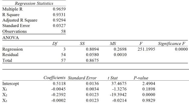
TABLE 13-15 The superintendent of a school district wanted to predict the percentage of students passing a sixth-grade proficiency test. She obtained the data on percentage of students passing the proficiency test (% Passing), daily mean of the percentage of students attending class (% Attendance), mean teacher salary in dollars (Salaries), and instructional spending per pupil in dollars (Spending) of 47 schools in the state. Following is the multiple regression output with Y = % Passing as the dependent variable, = : % Attendance, = Salaries and = Spending: 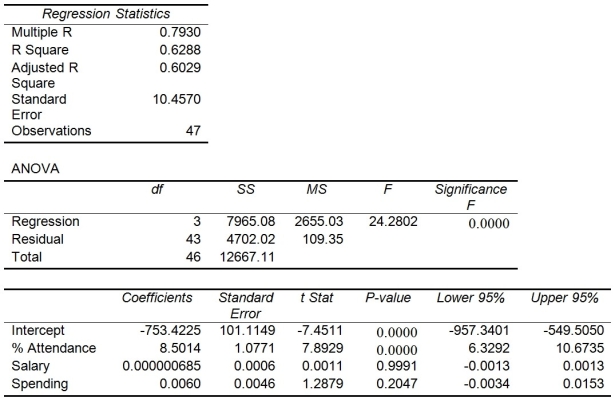-Referring to Table 13-15, you can conclude that instructional spending per pupil individually has no impact on the mean percentage of students passing the proficiency test, taking into account the effect of all the other independent variables, at a 1% level of significance based solely on the 95% confidence interval estimate for β₃.

TABLE 13-8 A financial analyst wanted to examine the relationship between salary (in $1,000) and four variables: age (X1 = Age), experience in the field (X2 = Exper), number of degrees (X3 = Degrees), and number of previous jobs in the field (X4 = Prevjobs). He took a sample of 20 employees and obtained the following Microsoft Excel output: 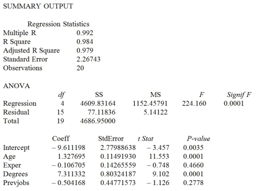-Referring to Table 13-8, the analyst decided to construct a 99% confidence interval for β₃. The confidence interval is from ________ to ________.

TABLE 13-10 You worked as an intern at We Always Win Car Insurance Company last summer. You noticed that individual car insurance premiums depend very much on the age of the individual, the number of traffic tickets received by the individual, and the population density of the city in which the individual lives. You performed a regression analysis in Microsoft Excel and obtained the following information: 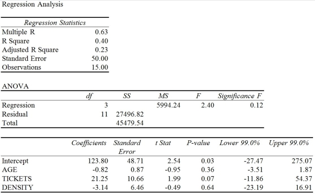-Referring to Table 13-10, the residual mean squares (MSE)that are missing in the ANOVA table should be ________.

TABLE 13-17 Given below are results from the regression analysis where the dependent variable is the number of weeks a worker is unemployed due to a layoff (Unemploy) and the independent variables are the age of the worker (Age), the number of years of education received (Edu), the number of years at the previous job (Job Yr), a dummy variable for marital status (Married: 1 = married, 0 = otherwise), a dummy variable for head of household (Head: 1 = yes, 0 = no) and a dummy variable for management position (Manager: 1 = yes, 0 = no). We shall call this Model 1. Model 2 is the regression analysis where the dependent variable is Unemploy and the independent variables are Age and Manager. The results of the regression analysis are given below: -Referring to Table 13-17 Model 1, there is sufficient evidence that all of the explanatory variables are related to the number of weeks a worker is unemployed due to a layoff at a 10% level of significance.

TABLE 13-15 The superintendent of a school district wanted to predict the percentage of students passing a sixth-grade proficiency test. She obtained the data on percentage of students passing the proficiency test (% Passing), daily mean of the percentage of students attending class (% Attendance), mean teacher salary in dollars (Salaries), and instructional spending per pupil in dollars (Spending) of 47 schools in the state. Following is the multiple regression output with Y = % Passing as the dependent variable, = : % Attendance, = Salaries and = Spending: -Referring to Table 13-15, predict the percentage of students passing the proficiency test for a school which has a daily mean of 95% of students attending class, a mean teacher salary of 40,000 dollars, and an instructional spending per pupil of 2,000 dollars.

TABLE 13-17 Given below are results from the regression analysis where the dependent variable is the number of weeks a worker is unemployed due to a layoff (Unemploy) and the independent variables are the age of the worker (Age), the number of years of education received (Edu), the number of years at the previous job (Job Yr), a dummy variable for marital status (Married: 1 = married, 0 = otherwise), a dummy variable for head of household (Head: 1 = yes, 0 = no) and a dummy variable for management position (Manager: 1 = yes, 0 = no). We shall call this Model 1. Model 2 is the regression analysis where the dependent variable is Unemploy and the independent variables are Age and Manager. The results of the regression analysis are given below: -Referring to Table 13-17 Model 1, there is sufficient evidence that age has an effect on the number of weeks a worker is unemployed due to a layoff, while holding constant the effect of all the other independent variables at a 10% level of significance.

TABLE 13-12 As a project for his business statistics class, a student examined the factors that determined parking meter rates throughout the campus area. Data were collected for the price per hour of parking, blocks to the quadrangle, and one of the three jurisdictions: on campus, in downtown and off campus, or outside of downtown and off campus. The population regression model hypothesized is Yi = α + β1X1i + β2X2i + β3X3i + ε where Y is the meter price X1 is the number of blocks to the quad X2 is a dummy variable that takes the value 1 if the meter is located in downtown and off campus and the value 0 otherwise X3 is a dummy variable that takes the value 1 if the meter is located outside of downtown and off campus, and the value 0 otherwise The following Microsoft Excel results are obtained. -Referring to Table 13-12, predict the meter rate per hour if one parks outside of downtown and off campus three blocks from the quad.

TABLE 13-10 You worked as an intern at We Always Win Car Insurance Company last summer. You noticed that individual car insurance premiums depend very much on the age of the individual, the number of traffic tickets received by the individual, and the population density of the city in which the individual lives. You performed a regression analysis in Microsoft Excel and obtained the following information: -A dummy variable is used as an independent variable in a regression model when

TABLE 13-10 You worked as an intern at We Always Win Car Insurance Company last summer. You noticed that individual car insurance premiums depend very much on the age of the individual, the number of traffic tickets received by the individual, and the population density of the city in which the individual lives. You performed a regression analysis in Microsoft Excel and obtained the following information: -Referring to Table 13-10, the total degrees of freedom that are missing in the ANOVA table should be ________.

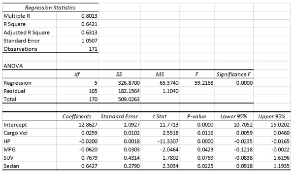
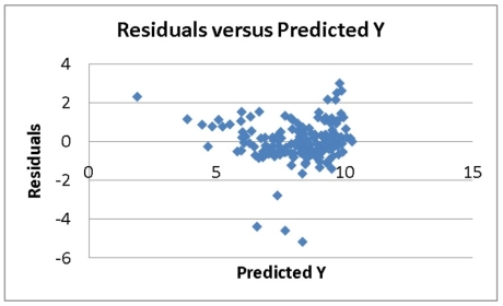
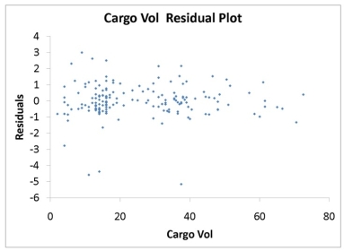
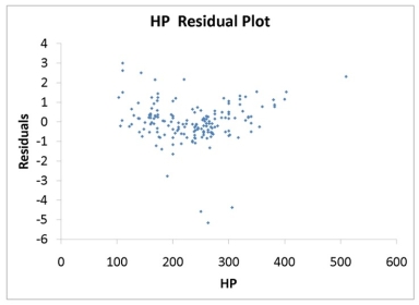
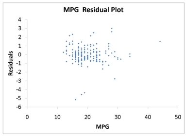
TABLE 13-16 What are the factors that determine the acceleration time (in sec.) from 0 to 60 miles per hour of a car? Data on the following variables for 171 different vehicle models were collected: Accel Time: Acceleration time in sec. Cargo Vol: Cargo volume in cu. ft. HP: Horsepower MPG: Miles per gallon SUV: 1 if the vehicle model is an SUV with Coupe as the base when SUV and Sedan are both 0 Sedan: 1 if the vehicle model is a sedan with Coupe as the base when SUV and Sedan are both 0 The regression results using acceleration time as the dependent variable and the remaining variables as the independent variables are presented below. The various residual plots are as shown below. 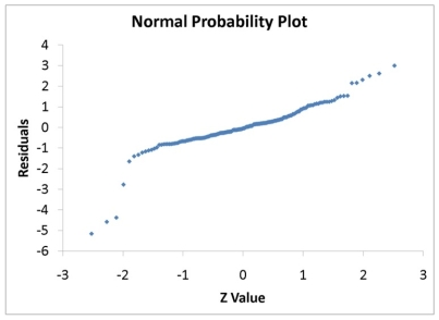The coefficient of multiple determination for the regression model using each of the 5 variables Xj as the dependent variable and all other X variables as independent variables (Rj2) are, respectively, 0.7461, 0.5676, 0.6764, 0.8582, 0.6632. -Referring to Table 13-16, which of the following assumptions is most likely violated based on the normal probability plot?