Exam 13: Introduction to Multiple Regression

TABLE 13-10 You worked as an intern at We Always Win Car Insurance Company last summer. You noticed that individual car insurance premiums depend very much on the age of the individual, the number of traffic tickets received by the individual, and the population density of the city in which the individual lives. You performed a regression analysis in Microsoft Excel and obtained the following information: 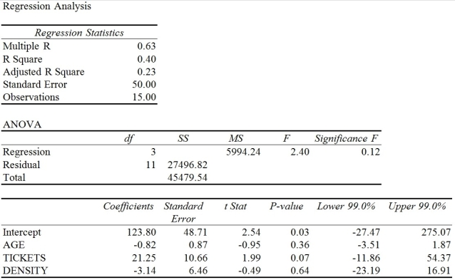-Referring to Table 13-10, to test the significance of the multiple regression model, what are the degrees of freedom?

TABLE 13-15 The superintendent of a school district wanted to predict the percentage of students passing a sixth-grade proficiency test. She obtained the data on percentage of students passing the proficiency test (% Passing), daily mean of the percentage of students attending class (% Attendance), mean teacher salary in dollars (Salaries), and instructional spending per pupil in dollars (Spending) of 47 schools in the state. Following is the multiple regression output with Y = % Passing as the dependent variable, = : % Attendance, = Salaries and = Spending: 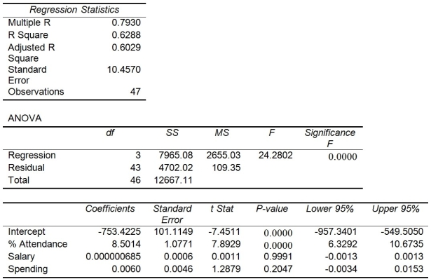-Referring to Table 13-15, which of the following is the correct alternative hypothesis to test whether daily mean of the percentage of students attending class has any effect on percentage of students passing the proficiency test, taking into account the effect of all the other independent variables?

TABLE 13-4 A real estate builder wishes to determine how house size (House) is influenced by family income (Income), family size (Size), and education of the head of household (School). House size is measured in hundreds of square feet, income is measured in thousands of dollars, and education is in years. The builder randomly selected 50 families and ran the multiple regression. Microsoft Excel output is provided below: 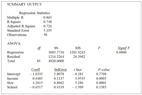-Referring to Table 13-4, suppose the builder wants to test whether the coefficient on Income is significantly different from 0. What is the value of the relevant t-statistic?

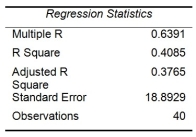
TABLE 13-17 Given below are results from the regression analysis where the dependent variable is the number of weeks a worker is unemployed due to a layoff (Unemploy) and the independent variables are the age of the worker (Age), the number of years of education received (Edu), the number of years at the previous job (Job Yr), a dummy variable for marital status (Married: 1 = married, 0 = otherwise), a dummy variable for head of household (Head: 1 = yes, 0 = no) and a dummy variable for management position (Manager: 1 = yes, 0 = no). We shall call this Model 1. 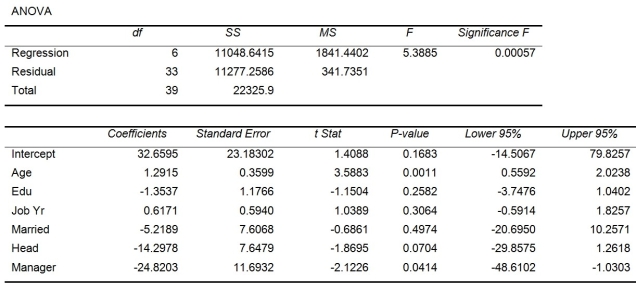Model 2 is the regression analysis where the dependent variable is Unemploy and the independent variables are Age and Manager. The results of the regression analysis are given below: -Referring to Table 13-17 Model 1, the alternative hypothesis H₁: At least one of βⱼ ≠ 0 for j = 1, 2, 3, 4, 5, 6 implies that the number of weeks a worker is unemployed due to a layoff is affected by all of the explanatory variables.

TABLE 13-13 An econometrician is interested in evaluating the relationship of demand for building materials to mortgage rates in Los Angeles and San Francisco. He believes that the appropriate model is Y = 10 + 5X1 + 8X2 where X1 = mortgage rate in % X2 = 1 if SF, 0 if LA Y = demand in $100 per capita -Referring to Table 13-13, the fitted model for predicting demand in Los Angeles is ________.

TABLE 13-16 What are the factors that determine the acceleration time (in sec.) from 0 to 60 miles per hour of a car? Data on the following variables for 171 different vehicle models were collected: Accel Time: Acceleration time in sec. Cargo Vol: Cargo volume in cu. ft. HP: Horsepower MPG: Miles per gallon SUV: 1 if the vehicle model is an SUV with Coupe as the base when SUV and Sedan are both 0 Sedan: 1 if the vehicle model is a sedan with Coupe as the base when SUV and Sedan are both 0 The regression results using acceleration time as the dependent variable and the remaining variables as the independent variables are presented below. 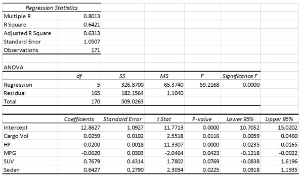The various residual plots are as shown below. 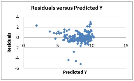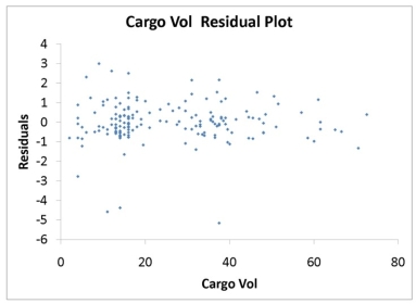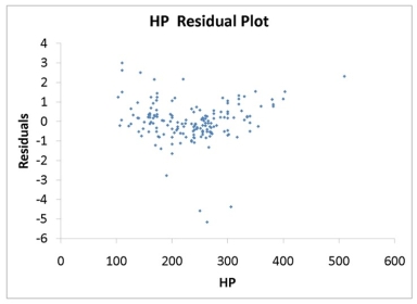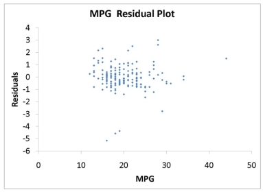The coefficient of multiple determination for the regression model using each of the 5 variables Xj as the dependent variable and all other X variables as independent variables (Rj2) are, respectively, 0.7461, 0.5676, 0.6764, 0.8582, 0.6632. -Referring to Table 13-16, which of the following assumptions is most likely violated based on the residual plot for HP?

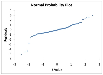
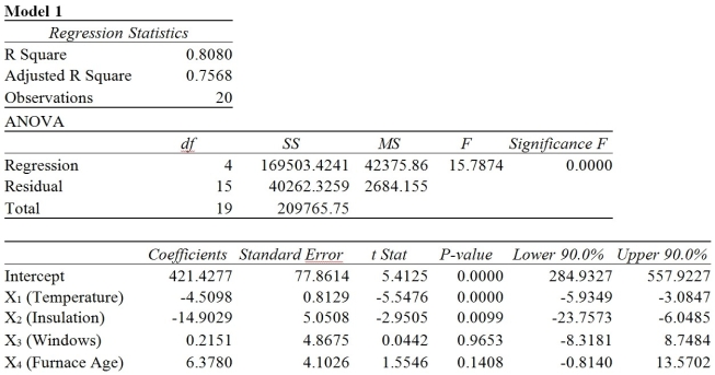
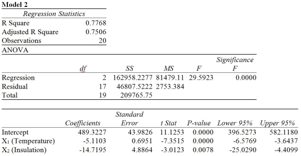
TABLE 13-6 One of the most common questions of prospective house buyers pertains to the cost of heating in dollars (Y). To provide its customers with information on that matter, a large real estate firm used the following four variables to predict heating costs: the daily minimum outside temperature in degrees of Fahrenheit (X1), the amount of insulation in inches (X2), the number of windows in the house (X3), and the age of the furnace in years (X4). Given below are the Microsoft Excel outputs of two regression models. -The slopes in a multiple regression model are called net regression coefficients.

TABLE 13-15 The superintendent of a school district wanted to predict the percentage of students passing a sixth-grade proficiency test. She obtained the data on percentage of students passing the proficiency test (% Passing), daily mean of the percentage of students attending class (% Attendance), mean teacher salary in dollars (Salaries), and instructional spending per pupil in dollars (Spending) of 47 schools in the state. Following is the multiple regression output with Y = % Passing as the dependent variable, = : % Attendance, = Salaries and = Spending: -Referring to Table 13-15, you can conclude that instructional spending per pupil individually has no impact on the mean percentage of students passing the proficiency test, taking into account the effect of all the other independent variables, at a 10% level of significance based solely on the 95% confidence interval estimate for β₃.

TABLE 13-17 Given below are results from the regression analysis where the dependent variable is the number of weeks a worker is unemployed due to a layoff (Unemploy) and the independent variables are the age of the worker (Age), the number of years of education received (Edu), the number of years at the previous job (Job Yr), a dummy variable for marital status (Married: 1 = married, 0 = otherwise), a dummy variable for head of household (Head: 1 = yes, 0 = no) and a dummy variable for management position (Manager: 1 = yes, 0 = no). We shall call this Model 1. Model 2 is the regression analysis where the dependent variable is Unemploy and the independent variables are Age and Manager. The results of the regression analysis are given below: -Referring to Table 13-17 Model 1, predict the number of weeks being unemployed due to a layoff for a worker who is a thirty-year-old, has 10 years of education, has 15 years of experience at the previous job, is married, is the head of household, and is a manager.

TABLE 13-3 An economist is interested to see how consumption for an economy (in $billions) is influenced by gross domestic product ($billions) and aggregate price (consumer price index). The Microsoft Excel output of this regression is partially reproduced below. 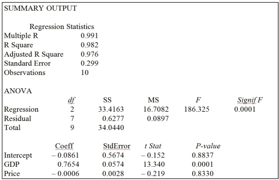-Referring to Table 13-3, to test whether gross domestic product has a positive impact on consumption, the p-value is ________.

TABLE 13-17 Given below are results from the regression analysis where the dependent variable is the number of weeks a worker is unemployed due to a layoff (Unemploy) and the independent variables are the age of the worker (Age), the number of years of education received (Edu), the number of years at the previous job (Job Yr), a dummy variable for marital status (Married: 1 = married, 0 = otherwise), a dummy variable for head of household (Head: 1 = yes, 0 = no) and a dummy variable for management position (Manager: 1 = yes, 0 = no). We shall call this Model 1. Model 2 is the regression analysis where the dependent variable is Unemploy and the independent variables are Age and Manager. The results of the regression analysis are given below: -Referring to Table 13-17 Model 1, what is the value of the test statistic when testing whether age has any effect on the number of weeks a worker is unemployed due to a layoff, while holding constant the effect of all the other independent variables?

TABLE 13-7 The department head of the accounting department wanted to see if she could predict the GPA of students using the number of course units (credits) and total SAT scores of each. She takes a sample of students and generates the following Microsoft Excel output: 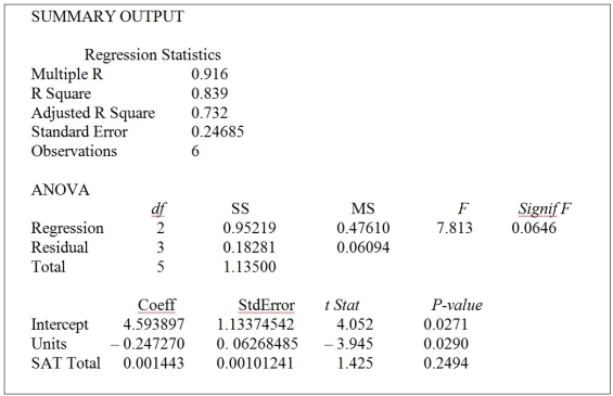-Referring to Table 13-7, the net regression coefficient of X₂ is ________.

TABLE 13-3 An economist is interested to see how consumption for an economy (in $billions) is influenced by gross domestic product ($billions) and aggregate price (consumer price index). The Microsoft Excel output of this regression is partially reproduced below. -Referring to Table 13-3, to test whether aggregate price index has a negative impact on consumption, the p-value is ________.

TABLE 13-15 The superintendent of a school district wanted to predict the percentage of students passing a sixth-grade proficiency test. She obtained the data on percentage of students passing the proficiency test (% Passing), daily mean of the percentage of students attending class (% Attendance), mean teacher salary in dollars (Salaries), and instructional spending per pupil in dollars (Spending) of 47 schools in the state. Following is the multiple regression output with Y = % Passing as the dependent variable, = : % Attendance, = Salaries and = Spending: -Referring to Table 13-15, there is sufficient evidence that all of the explanatory variables are related to the percentage of students passing the proficiency test at a 5% level of significance.

TABLE 13-12 As a project for his business statistics class, a student examined the factors that determined parking meter rates throughout the campus area. Data were collected for the price per hour of parking, blocks to the quadrangle, and one of the three jurisdictions: on campus, in downtown and off campus, or outside of downtown and off campus. The population regression model hypothesized is Yi = α + β1X1i + β2X2i + β3X3i + ε where Y is the meter price X1 is the number of blocks to the quad X2 is a dummy variable that takes the value 1 if the meter is located in downtown and off campus and the value 0 otherwise X3 is a dummy variable that takes the value 1 if the meter is located outside of downtown and off campus, and the value 0 otherwise The following Microsoft Excel results are obtained. -An interaction term in a multiple regression model may be used when the relationship between X₁ and Y changes for differing values of X₂.

TABLE 13-17 Given below are results from the regression analysis where the dependent variable is the number of weeks a worker is unemployed due to a layoff (Unemploy) and the independent variables are the age of the worker (Age), the number of years of education received (Edu), the number of years at the previous job (Job Yr), a dummy variable for marital status (Married: 1 = married, 0 = otherwise), a dummy variable for head of household (Head: 1 = yes, 0 = no) and a dummy variable for management position (Manager: 1 = yes, 0 = no). We shall call this Model 1. Model 2 is the regression analysis where the dependent variable is Unemploy and the independent variables are Age and Manager. The results of the regression analysis are given below: -Referring to Table 13-17 Model 1, we can conclude that, holding constant the effect of the other independent variables, there is a difference in the mean number of weeks a worker is unemployed due to a layoff between a worker who is married and one who is not at a 10% level of significance if we use only the information of the 95% confidence interval estimate for β₄.

TABLE 13-15 The superintendent of a school district wanted to predict the percentage of students passing a sixth-grade proficiency test. She obtained the data on percentage of students passing the proficiency test (% Passing), daily mean of the percentage of students attending class (% Attendance), mean teacher salary in dollars (Salaries), and instructional spending per pupil in dollars (Spending) of 47 schools in the state. Following is the multiple regression output with Y = % Passing as the dependent variable, = : % Attendance, = Salaries and = Spending: -Referring to Table 13-15, which of the following is the correct null hypothesis to determine whether there is a significant relationship between percentage of students passing the proficiency test and the entire set of explanatory variables?

TABLE 13-6 One of the most common questions of prospective house buyers pertains to the cost of heating in dollars (Y). To provide its customers with information on that matter, a large real estate firm used the following four variables to predict heating costs: the daily minimum outside temperature in degrees of Fahrenheit (X1), the amount of insulation in inches (X2), the number of windows in the house (X3), and the age of the furnace in years (X4). Given below are the Microsoft Excel outputs of two regression models. -Referring to Table 13-6, what is your decision and conclusion for the test H₀: β₂ = 0 vs. H₁: β₂ < 0 at the α = 0.01 level of significance using Model 1?

TABLE 13-6 One of the most common questions of prospective house buyers pertains to the cost of heating in dollars (Y). To provide its customers with information on that matter, a large real estate firm used the following four variables to predict heating costs: the daily minimum outside temperature in degrees of Fahrenheit (X1), the amount of insulation in inches (X2), the number of windows in the house (X3), and the age of the furnace in years (X4). Given below are the Microsoft Excel outputs of two regression models. -When an explanatory variable is dropped from a multiple regression model, the coefficient of multiple determination can increase.

TABLE 13-6 One of the most common questions of prospective house buyers pertains to the cost of heating in dollars (Y). To provide its customers with information on that matter, a large real estate firm used the following four variables to predict heating costs: the daily minimum outside temperature in degrees of Fahrenheit (X1), the amount of insulation in inches (X2), the number of windows in the house (X3), and the age of the furnace in years (X4). Given below are the Microsoft Excel outputs of two regression models. -A multiple regression is called "multiple" because it has several explanatory variables.